高维可视化方法

t-SNE

t-SNE是数据降维与可视化方法，但是它的缺点也很明显，比如：占内存大，运行时间长。

但是，当我们想要对高维数据进行分类，又不清楚这个数据集有没有很好的可分性（即同类之间间隔小，异类之间间隔大），可以通过t-SNE投影到2维或者3维的空间中观察一下。如果在低维空间中具有可分性，则数据是可分的；如果在高维空间中不具有可分性，可能是数据不可分，也可能仅仅是因为不能投影到低维空间。

原理

t-SNE（TSNE）将数据点之间的相似度转换为概率。原始空间中的相似度由高斯联合概率表示，嵌入空间的相似度由“学生t分布”表示。

实例

# coding='utf-8'
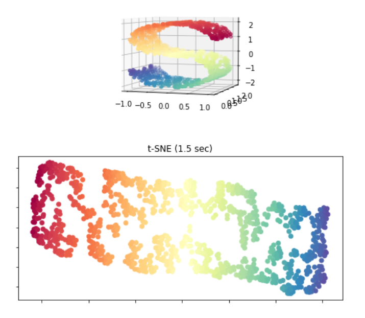
"""# 一个对S曲线数据集上进行各种降维的说明。"""
from time import time

import matplotlib.pyplot as plt
from mpl_toolkits.mplot3d import Axes3D
from matplotlib.ticker import NullFormatter

from sklearn import manifold, datasets

# # Next line to silence pyflakes. This import is needed.
# Axes3D

n_points = 1000
# X是一个(1000, 3)的2维数据，color是一个(1000,)的1维数据
X, color = datasets.make_s_curve(n_points, random_state=0)
n_neighbors = 10
n_components = 2

fig = plt.figure(figsize=(8, 8))
# 创建了一个figure，标题为"Manifold Learning with 1000 points, 10 neighbors"
plt.suptitle("Manifold Learning with %i points, %i neighbors"
             % (1000, n_neighbors), fontsize=14)


'''绘制S曲线的3D图像'''
ax = fig.add_subplot(211, projection='3d')
ax.scatter(X[:, 0], X[:, 1], X[:, 2], c=color, cmap=plt.cm.Spectral)
ax.view_init(4, -72)  # 初始化视角

'''t-SNE'''
t0 = time()
tsne = manifold.TSNE(n_components=n_components, init='pca', random_state=0)
Y = tsne.fit_transform(X)  # 转换后的输出
t1 = time()
print("t-SNE: %.2g sec" % (t1 - t0))  # 算法用时
ax = fig.add_subplot(2, 1, 2)
plt.scatter(Y[:, 0], Y[:, 1], c=color, cmap=plt.cm.Spectral)
plt.title("t-SNE (%.2g sec)" % (t1 - t0))
ax.xaxis.set_major_formatter(NullFormatter())  # 设置标签显示格式为空
ax.yaxis.set_major_formatter(NullFormatter())
# plt.axis('tight')

plt.show()

UMAP

由于UMAP能够同时保留数据中的局部和全局结构，它被选为最有效的降维方法。与PCA和t-SNE相比，UMAP提供了最好的分类结果可视化。UMAP不仅保留了数据点之间的局部关系，还确保了全局结构（不同矿床类型的广泛分组）的保留，这使得它在分析复杂数据集时非常有效。它的高效性使其特别适合处理大数据集.

原理

实例