python一对一辅导教程：Computational Problems for Physics chapter 1-A Code Listings 1.1 - 1.6

关注

原创最新推荐文章于 2026-05-05 09:54:46 发布 502 阅读 AI 写同款· GEO 优化 ›

Computational-physics:计算物理例程计算物理学 C语言中的计算物理例程内容使用梯形规则实现的集成，支持具有自定义参数的功能立即下载

作者自我介绍：大爽歌, b站小UP主，直播编程+红警三，python1对1辅导老师。
本博客为一对一辅导学生python代码的教案, 获得学生允许公开。
具体辅导内容为《Computational Problems for Physics With Guided Solutions Using Python》，第一章（Chapter 1 Computational Basics for Physics）的 Code Listings
由于代码较多，第一章内容分为三部分
A(1.1 - 1.6)
B(1.7 - 1.11)
C(1.12 - 1.17)

0 安装第三方库

已安装

numpy
matplotlib

待安装

vpython
pylab (a tool from matplotlib)
mpl_toolkits (a tool from matplotlib)
visual (unknown)

pip install VPython -i https://pypi.tuna.tsinghua.edu.cn/simple
pip install matplotlib -i https://pypi.tuna.tsinghua.edu.cn/simple

参考书（链接）：

https://www.glowscript.org/docs/VPythonDocs/graph.html

1 - vpython graph

uses VPython to produce the two plots in Figure 1.1.

graph

a graph is inherently 2D and contains graphing objects for displaying curves, dots, and vertical or horizontal bars.
粗略中文理解，一片2D区域，展示graphing objects，像画板一样

如果不设置graph，代码里面的图会绘制到vpython的默认初始graph（自带的）中
设置了graph后，代码里面的图会绘制到它最近的上面的那个graph中

以下展示了两个graph对象

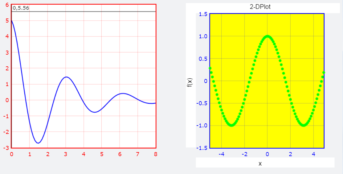
生成该图的代码如下

from vpython import *  # EasyVisualVP.py


graph1=graph(align='left',width=400,height=400, background=color.white,foreground=color.red)

Plot1=gcurve(color=color.blue)  # gcurve method
for x in arange(0,8.1,0.1):  # xrange
    Plot1.plot(pos=(x,5*cos(2*x)*exp(-0.4*x)))

graph2=graph(align='right',width=400,height=400,
             background=color.yellow,foreground=color.blue,
             title='2-DPlot',xtitle='x',ytitle='f(x)')

Plot2=gdots(color=color.green)  # Dots
for x in arange(-5,5,0.1):
    Plot2.plot(pos=(x,cos(x)))  # plotdots

我们提取出上面代码中，生成两个graph对象的生成代码来观察下

graph1=graph(align='left', width=400, height=400, 
             background=color.white, foreground=color.red)
graph2=graph(align='right',width=400, height=400,
             background=color.yellow, foreground=color.blue,
             title='2-DPlot', xtitle='x', ytitle='f(x)')

graph是一个class，创建graph对象代码中的参数意思

align 对齐方式只能是以下三个值之一
'left', 'right', or 'none'(the default).
width 宽度
height 高度
background 背景色
foreground 前景色(方框和xy轴的刻度颜色)
title 图标题
xtitle x轴的标题
ytitle y轴的标题

参数拓展（上面只展示了graph刚才用的的参数，graph所有参数如下）

# from vpython.py :2253
scalarAttributes = ['width', 'height', 'title', 'xtitle', 'ytitle','align',
'xmin', 'xmax', 'ymin', 'ymax', 'logx', 'logy', 'fast', 'scroll']

2 - vpython graph plotting objects

gcurve: a connected curve 连通的曲线
gdots: disconnected dots 散点
gvbars: vertical bars 垂直条
ghbars: horizontal bars 水平条

使用对应的方法，将会根据设置的样式生成具有该样式的plotting

比如Plot1=gcurve(color=color.blue)就会生成一个颜色为蓝色的连通的曲线gcurve。

这个时候曲线上是没有内容的，即没有点。

比如运行以下两行代码，会生成一个空白页面（因为没有内容）

from vpython import *  # Import Vpython
Plot1=gcurve(color=color.blue)

给这个曲线加点的方法如下（简单写法，这个里面参数可能还有可以拓展说明的，具体后面遇到再说）
Plot1.plot(pos=(x,y))

一般会使用循环来添加，例如for x in arange(start, end, step)。

其中arange, 是来自numpy的函数。

这个函数比range好，因为支持float浮点数（range不支持）。

这里展示下上面四种类型的plotting objects的效果，如下

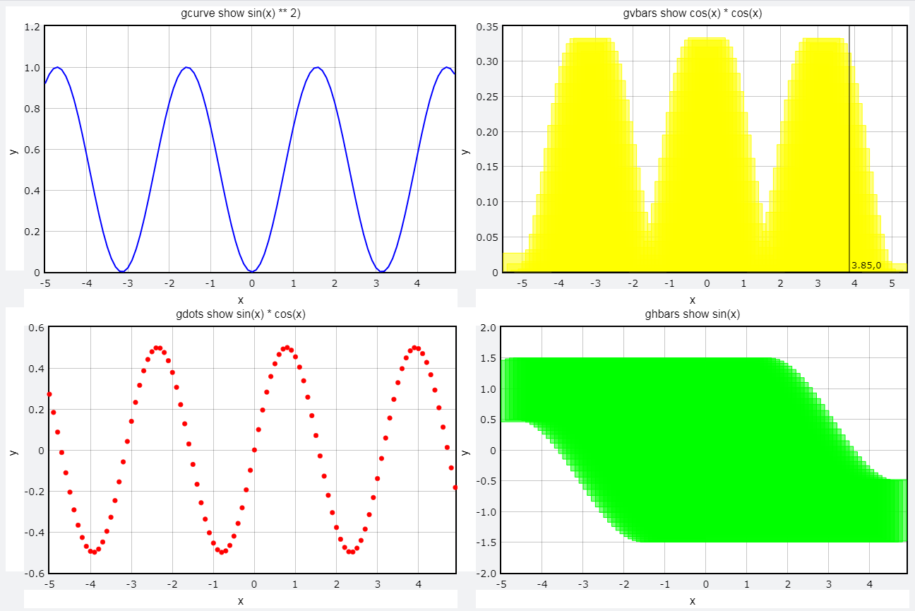
对应代码为

from vpython import *  # changed from 3GraphVP.py

graph(align='left', title="gcurve show sin(x) ** 2)", xtitle='x', ytitle='y', background=color.white, foreground=color.black)
y1 = gcurve(color=color.blue)
for x in arange(-5, 5, 0.1):
    y1.plot(pos=(x, sin(x) ** 2))

graph(align='left',title="gvbars show cos(x) * cos(x)", xtitle='x', ytitle='y', background=color.white, foreground=color.black)
y2 = gvbars(color=color.yellow)

for x in arange(-5, 5, 0.1):
    y2.plot(pos=(x, cos(x) * cos(x) / 3.))

graph(align='left',title="gdots show sin(x) * cos(x)", xtitle='x', ytitle='y', background=color.white, foreground=color.black)
y3 = gdots(color=color.red)

for x in arange(-5, 5, 0.1):
    y3.plot(pos=(x, sin(x) * cos(x)))

graph(align='left',title="ghbars show sin(x)", xtitle='x', ytitle='y', background=color.white, foreground=color.black)
y4 = ghbars(color=color.green)

for x in arange(-5, 5, 0.1):
    y4.plot(pos=(x, sin(x)))

3 - vpython 中的一些其他常用变量

`color`

颜色，包含以下几个值
black、white、red、green、blue、
yellow、cyan、magenta、orange、purple

其他包（Package)

vpython里面包含了其他包，比如numpy，所以上面的代码才可以直接写arange, sin等函数。

这里展示下包含的常用包方法

math.*
包含sin, cos等等
numpy.arange
random.random

4 - numpy array

The array object in NumPy is called ndarray.

可以用列表创建，也常用np.arange(Xmin, Xmax, DelX)方法来创建

数组很像列表，但比里列表强大，强在支持各种运算
比如下面的

import numpy as np  # a part from EasyMatPlot.py


Xmin = -5.;    Xmax = +5.;    Npoints = 20
DelX = (Xmax - Xmin) / Npoints

x = np.arange(Xmin, Xmax, DelX)
y = np.sin(x) * np.sin(x*x)
print(x)
# [-5.  -4.5 -4.  -3.5 -3.  -2.5 -2.  -1.5 -1.  -0.5  0.   0.5  1.   1.5  
# 2.   2.5  3.   3.5  4.   4.5]
print(y)
# [-0.12691531  0.96338048 -0.21788595 -0.10913545 -0.05815816  0.01985684
#   0.68815856 -0.77612411 -0.70807342 -0.11861178  0.          0.11861178
#   0.70807342  0.77612411 -0.68815856 -0.01985684  0.05815816  0.10913545
#   0.21788595 -0.96338048]

注意：numpy中也有sin、cos方法，
但是和math中的sin、cos方法不同，numpy中的支持数组运算。

pylab 对 numpy 的调用

pylab 中，对numpy进行了两次重要调用如下

from numpy import *
import numpy as np

所以在导入了pylab的代码中，使用np.arange和arange都是可以的。
需要注意的一点事，此时使用sin和cos等，都是来自numpy的支持数组运算的。

5 - 1.3 EasyMatPlot.py

1 占位符

详细文档：python 格式化输出详解上篇

占位符格式

”%s“ % variable 一个
”%s %s %s“ % (a, b, c) 多个

具体到EasyMatPlot.py的代码中的
”%8.2f“ % x[0]的%8.2f

8是width，占位符总宽度（字符、数字个数）
.2 是精度设置，代表精度为2，可以理解为保留2位小数
f 代表格式为浮点数

运行效果如下

y = [196338.048,-0.12691531,-78.8595,-581581.6]
print("%8.2f,%8.2f,%8.2f,%8.2f" % tuple(y))
# 196338.05,   -0.13,  -78.86,-581581.60

2 EasyMatPlot 绘制效果

其代码如下

from pylab import *  # EasyMatPlot.py

Xmin = -5. ;  Xmax = +5. ;  Npoints = 500 
DelX = (Xmax - Xmin) / Npoints

x = arange(Xmin, Xmax, DelX)
y = sin(x) * sin(x*x)

print("arange => x[0], x[1], x[499] = %8.2f %8.2f %8.2f" %(x[0], x[1], x[499]))
print("arange => y[0], y[1], y[499] = %8.2f %8.2f %8.2f" %(y[0], y[1], y[499]))

print("\n Doing plotting, look for Figure 1")

xlabel('x') ;  ylabel('f(x)') ;  title('f(x)vsx')
text(1.75, 0.75, 'MatPlotLib \n Example')
plot(x, y, '-', lw=2)
grid(True)
show()

绘制效果如图

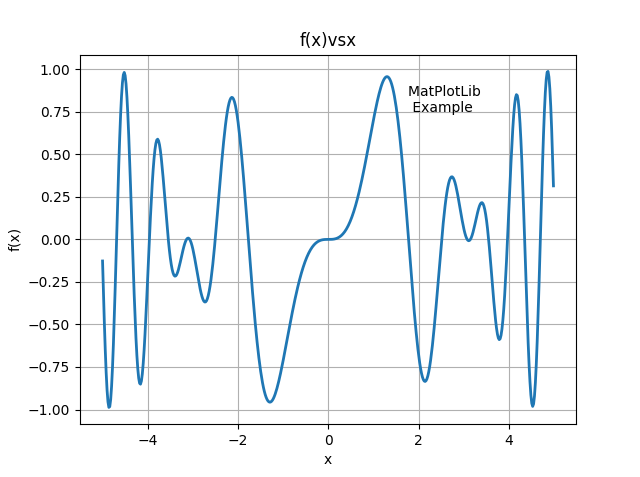
后半部分代码说明见下文（即第六部分）

6 - matplotlib

pylab中导入了 matplotlib 。
EasyMatPlot.py最后五行的代码使用的方法其实都是matplotlib.pyplot的方法
一般matplotlib都会导入pyplot为plt

1 函数简单介绍

xlabel 设置x轴文本
ylabel 设置y轴文本
title 设置图表标题
grid 是否展示网格
show 展示图表
text(x, y, s) 在图上坐标为(x,y)的地方展示文本s。

2 plot

详细文档： matplotlib.pyplot.plot

plot函数比较复杂，其详细参数格式如下

matplotlib.pyplot.plot(*args, scalex=True, scaley=True, data=None, **kwargs)

这里我们做一个简化的介绍，介绍一些常见的写法（可能还会有其他写法，遇到再说）
EasyMatPlot.py中的写法plot(x, y, '-', lw=2)，是一种比较常见的写法

plot([x], y, [fmt], *, data=None, **kwargs)
plot([x], y, [fmt], [x2], y2, [fmt2], ..., **kwargs)

其中

x 横坐标组成的列表（或数组），
y 纵坐标组成的列表（或数组）
fmt 定义基本格式(如颜色、标记和线型)，EasyMatPlot.py中的’-'代表线型为实线

fmt 只是快速设置基本属性的缩写。所有这些以及更多的都可以由关键字kwargs参数控制。

fmt 详细格式为[marker][line][color]

	说明	值举例
`marker`	标记（点的样式）	`'.'`、`'，'`、`'o'`、`'v'`、`'^'`、`'<'`、`'>'`、`'1'`、`'2'`、`'3'`、`'4'`
`line`	线的样式	`'-'`、`'--'`、`'-.'`、`':'`
`color`	颜色	`'r'`、`'g'`、`'b'`、`'c'`、`'m'`、`'y'`、`'k'`、`'w'`

将EasyMatPlot.py中绘图时的fmt设置为'o--r'，
效果如下图(标记点为圆点，线为虚线，颜色为color).

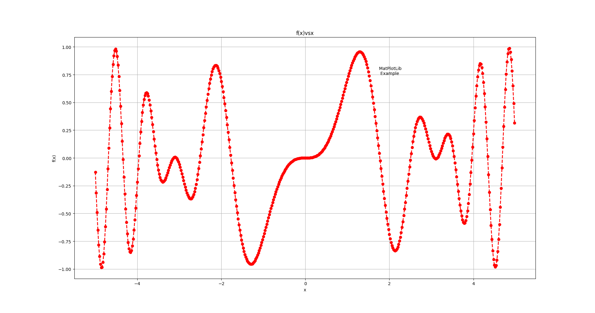
marker、line、color都是可选的，都不指定的话使用使用样式循环style cycle中的值
两点说明：
不指定marker的话，不展示点。
指定了marker不指定line的话，不展示线。

这个特性可以用来分别指定线和点。
fmt设置为'^b'

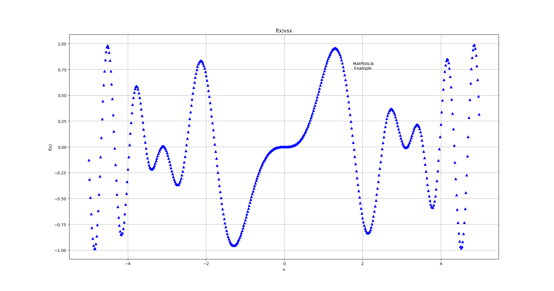
fmt设置为'-.g'

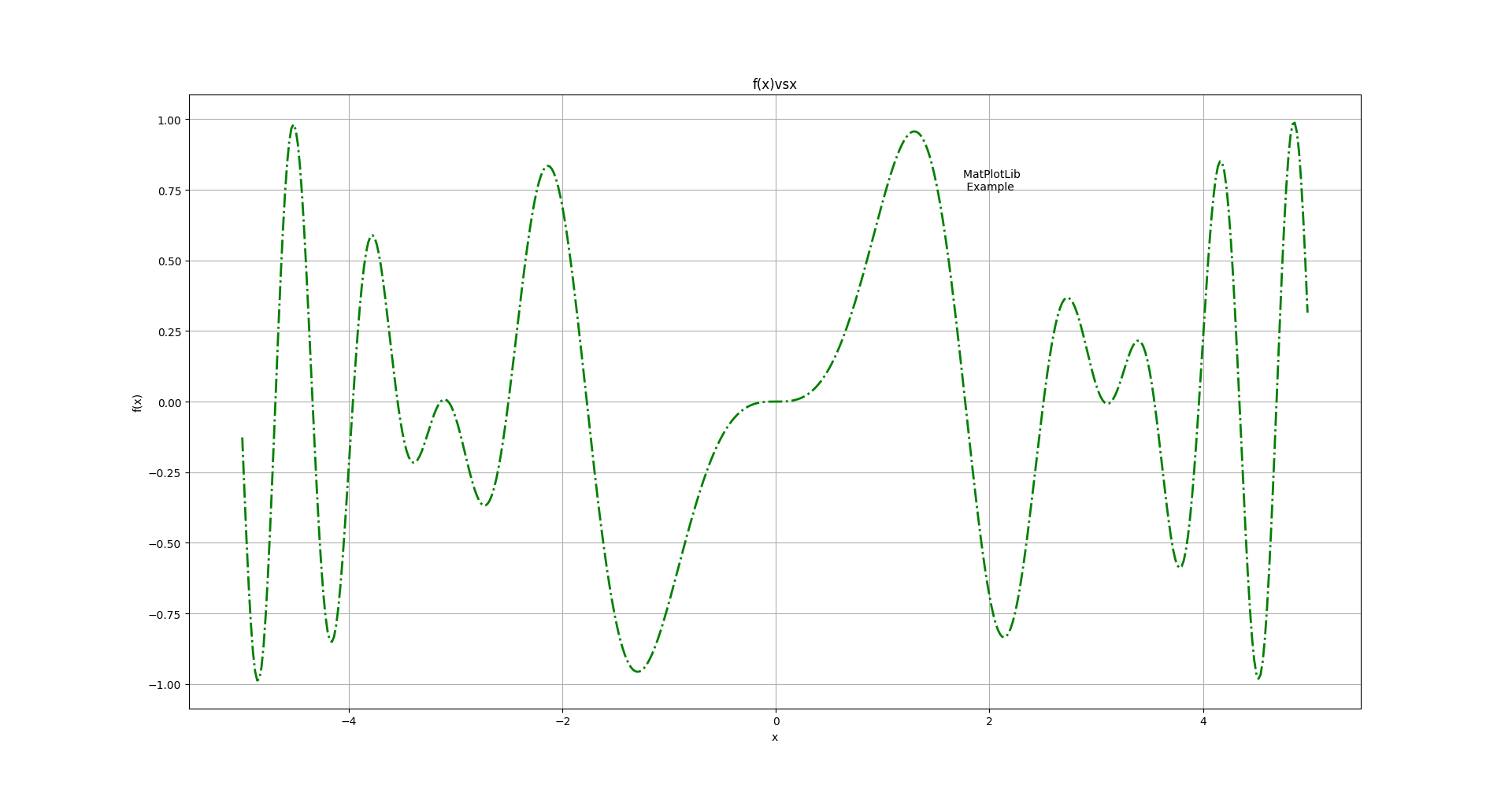
详细参数说明见官方文档
中的fmt部分

kwargs 设置一些keyword参数，EasyMatPlot.py中的lw=2代表线宽设置为2，等价于(linewidth=2)
详细参数说明见官方文档
中的kwargs部分

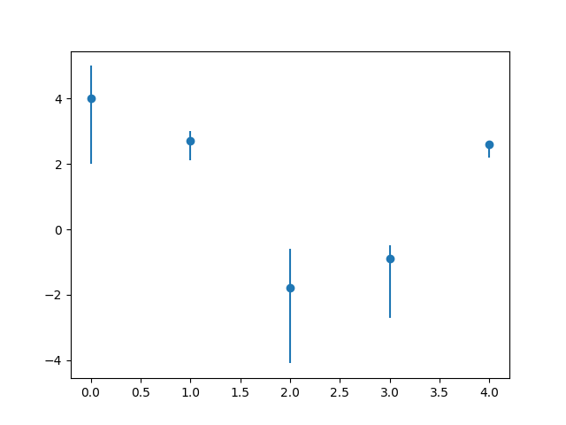
3 errorbar

Plot y versus x as lines and/or markers with attached errorbars.
from errorbar

具体效果为，在指定点绘制误差线（x轴或者y轴）

参数过多，简单写法为
matplotlib.pyplot.errorbar(x, y, yerr=None, xerr=None, fmt='', **kwargs)

yerr：指定平行于y轴的误差线范围（长度）
xerr：指定平行于x轴的误差线范围（长度）

其值格式相同，支持

scalar(a float): 对称加减值
shape(N,): 一维数组（N和x，y的N相同）,对称加减值
shape(2, N): 二维数组（N和x，y的N相同）, 分别指定加减值。
Separate - and + values for each bar. First row contains the lower errors, the second row contains the upper errors.
None: No errorbar.

import pylab as p
from numpy import *

x1 = arange(0, 5, 1)                    # Data set 1 points
y1 = array([4.0, 2.7, -1.8, -0.9, 2.6])
errTop = array([1.0, 0.3, 1.2, 0.4, 0.1]) # Asymm errors
errBot = array([2.0, 0.6, 2.3, 1.8, 0.4])
p.errorbar(x1, y1, [errBot, errTop], fmt = 'o') # Error bars

p.show()

效果如下图

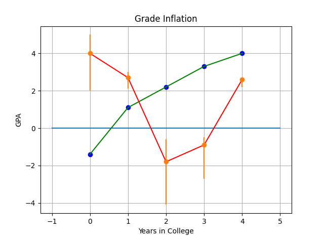
7 - 1.4 GradesMatPlot.py

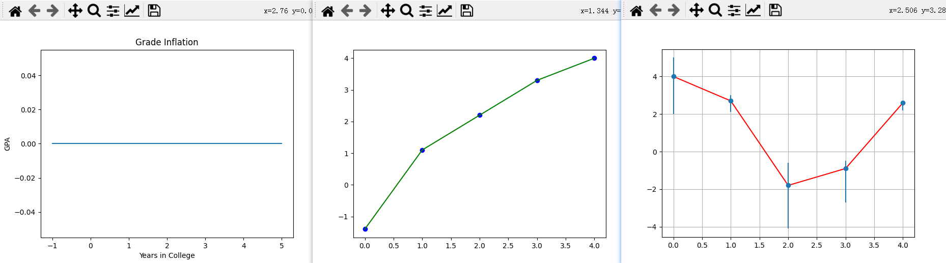
GradesMatPlot一张图里面绘了很多线，多了就乱，乱了就容易分不清哪个图是哪个代码产生的。

所以对代码分段，图分别绘制（中间show一次就是绘制了一次），
即代码如下

import pylab as p                           # Matplotlib
from numpy import *

p.title('Grade Inflation')           # Title and labels
p.xlabel('Years in College')
p.ylabel('GPA')
xa = array([-1, 5])                  # For horizontal line
ya = array([0, 0])
p.plot(xa, ya)                       # Draw horizontal line
p.show()   # draw 1 


x0 = array([0, 1, 2, 3, 4])            # Data set 0 points
y0 = array([-1.4, +1.1, 2.2, 3.3, 4.0])
p.plot(x0, y0, 'bo')            # Data set 0 = blue circles
p.plot(x0, y0, 'g')                     # Data set 0 = line
p.show()  # draw 2 


x1 = arange(0, 5, 1)                    # Data set 1 points
y1 = array([4.0, 2.7, -1.8, -0.9, 2.6])
p.plot(x1, y1, 'r')
errTop = array([1.0, 0.3, 1.2, 0.4, 0.1]) # Asymm errors
errBot = array([2.0, 0.6, 2.3, 1.8, 0.4])
p.errorbar(x1, y1, [errBot, errTop], fmt = 'o') # Error bars
p.grid(True)                                    # Grid line
p.show()  # draw 3

三次绘制效果如下图

GradesMatPlot.py中三图一起绘制，就是叠在一起，如下图

8 - 1.5 MatPlot2figs.py

1 figure

创建一个新的图形(窗口)，或者激活一个现有的图形，
返回一个matplotlib.figure.Figure对象，返回值有时会用到。

简单使用方法：

matplotlib.pyplot.figure(num=None)

num: 图形的唯一标识符，可以为数字(int)和字符串(string)。

如果具有该标识符的图形已经存在，则此图形将被激活并返回。
如果没有，就创建一个新的图形（窗口）。

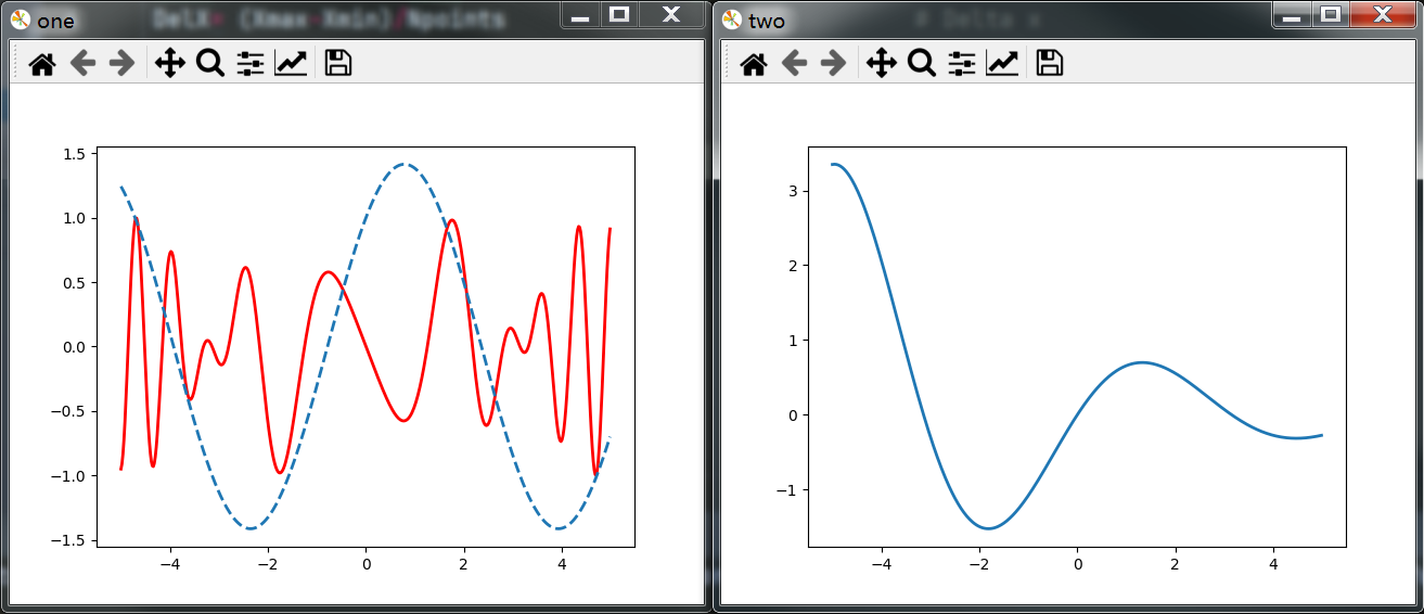
这里举一个代码的例子如下：

from pylab import *  # Simplified from MatPlot2figs.py

Xmin = -5.0;      Xmax =  5.0;        Npoints= 500
DelX= (Xmax-Xmin)/Npoints                             # Delta x
x1 = arange(Xmin, Xmax, DelX)                        # x1 range
y1 = -sin(x1)*cos(x1*x1)                           # Function 1
y2 = exp(-x1/4.)*sin(x1)
y3 = sin(x1) + cos(x1)

figure("one")
plot(x1, y1, 'r', lw=2)

figure("two")
plot(x1, y2, '-', lw=2)

figure("one")
plot(x1, y3, '--', lw=2)

show()

运行后效果如下（会同时打开两个窗口，后面的会挡住前面的，移动一下就好）

补充：
上面代码中的exp函数是numpy中的，
np.exp(x)代表计算e的x次方，
如果x是数组，则针对数组中的元素计算，生成新的数组。

2 subplot

作用：在当前图形figure上添加一个子图（划分出一个区域绘制子图）。
简单使用方法为subplot(nrows, ncols, index, **kwargs)

将figure划分为nrows行、ncols列个子图区域（此时每个区域内什么都没有），
在第index个区域创建子图并进行绘制（此时会在子图内绘制出初始坐标轴）。

index计算顺序为：从左到右，从上到下。

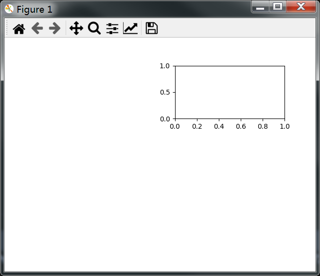
简单例子如下

from pylab import *

figure(1)
subplot(3,2,2)
show()

绘制效果图如下

3 MatPlot2figs 绘制效果

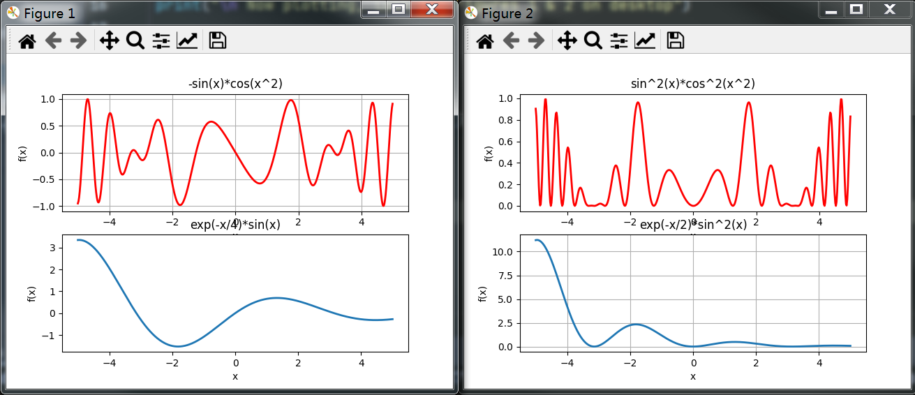
此时再看MatPlot2figs.py, 就很好看明白了。

from pylab import *      # MatPlot2figs.py

Xmin = -5.0;      Xmax =  5.0;        Npoints= 500
DelX= (Xmax-Xmin)/Npoints                             # Delta x
x1 = arange(Xmin, Xmax, DelX)                        # x1 range
x2 = arange(Xmin, Xmax, DelX/20)            # Different x2 range
y1 =  -sin(x1)*cos(x1*x1)                           # Function 1
y2 =   exp(-x2/4.)*sin(x2)                          # Function 2
print("\n Now plotting, look for Figures 1 & 2 on desktop")

figure(1)
subplot(2,1,1)                     # 1st subplot in first figure
plot(x1, y1, 'r', lw=2) 
xlabel('x');      ylabel( 'f(x)' ); title( '-sin(x)*cos(x^2)' )
grid(True)                                         # Form grid
subplot(2,1,2)                     # 2nd subplot in first figure
plot(x2, y2, '-', lw=2)
xlabel('x')                                        # Axes labels
ylabel( 'f(x)' )
title( 'exp(-x/4)*sin(x)' )

#                                  Figure 2 
figure(2)
subplot(2,1,1)                     # 1st subplot in 2nd figure
plot(x1, y1*y1, 'r', lw=2) 
xlabel('x'); ylabel('f(x)'); title('sin^2(x)*cos^2(x^2)') # grid
subplot(2,1,2)                       # 2nd subplot in 2nd figure
plot(x2, y2*y2, '-', lw=2)
xlabel('x');   ylabel( 'f(x)' );  title( 'exp(-x/2)*sin^2(x)' ) 
grid(True)
show()                                           # Show graphs

其绘制效果如图

9 - 1.6 Simple3Dplot.py

1 meshgrid

meshgrid是numpy中的方法，用于从坐标向量（一维）返回坐标矩阵（多维）。
简单写法为np.meshgrid(*xi)

*xi：*代表可以接受不定数量个参数，每个参数为表示网格坐标的一维数组。

x1, x2,…, xn array_like.
1-D arrays representing the coordinates of a grid.

代码示例

import numpy as np

delta = 0.5
x = np.arange( -2., 2., delta )
y = np.arange( -1., 1., delta )
X, Y = np.meshgrid(x, y)
Z = np.sin(X) * np.cos(Y)
print(X)
# [[-2.  -1.5 -1.  -0.5  0.   0.5  1.   1.5]
#  [-2.  -1.5 -1.  -0.5  0.   0.5  1.   1.5]
#  [-2.  -1.5 -1.  -0.5  0.   0.5  1.   1.5]
#  [-2.  -1.5 -1.  -0.5  0.   0.5  1.   1.5]]
print(Y)
# [[-1.  -1.  -1.  -1.  -1.  -1.  -1.  -1. ]
#  [-0.5 -0.5 -0.5 -0.5 -0.5 -0.5 -0.5 -0.5]
#  [ 0.   0.   0.   0.   0.   0.   0.   0. ]
#  [ 0.5  0.5  0.5  0.5  0.5  0.5  0.5  0.5]]
print(Z)
# [[-0.4912955  -0.53894884 -0.45464871 -0.25903472  0.          0.25903472  0.45464871  0.53894884]
#  [-0.79798357 -0.87538421 -0.73846026 -0.42073549  0.          0.42073549  0.73846026  0.87538421]
#  [-0.90929743 -0.99749499 -0.84147098 -0.47942554  0.          0.47942554  0.84147098  0.99749499]
#  [-0.79798357 -0.87538421 -0.73846026 -0.42073549  0.          0.42073549  0.73846026  0.87538421]]

直播间某位会matlab的观众弹幕补充（是否适用于matplotlib待确定）：
要绘制3d网格的话要3点坐标，必须使用2d网格。
如果只是绘制3D线条就不用了（不需要使用meshgrid)

2 Axes3D

mpl_toolkits.mplot3d.axes3d.Axes3D(fig, **kwargs)

绘制三维坐标轴，返回一个坐标轴对象。

Simple3Dplot.py中，该对象用到的方法：

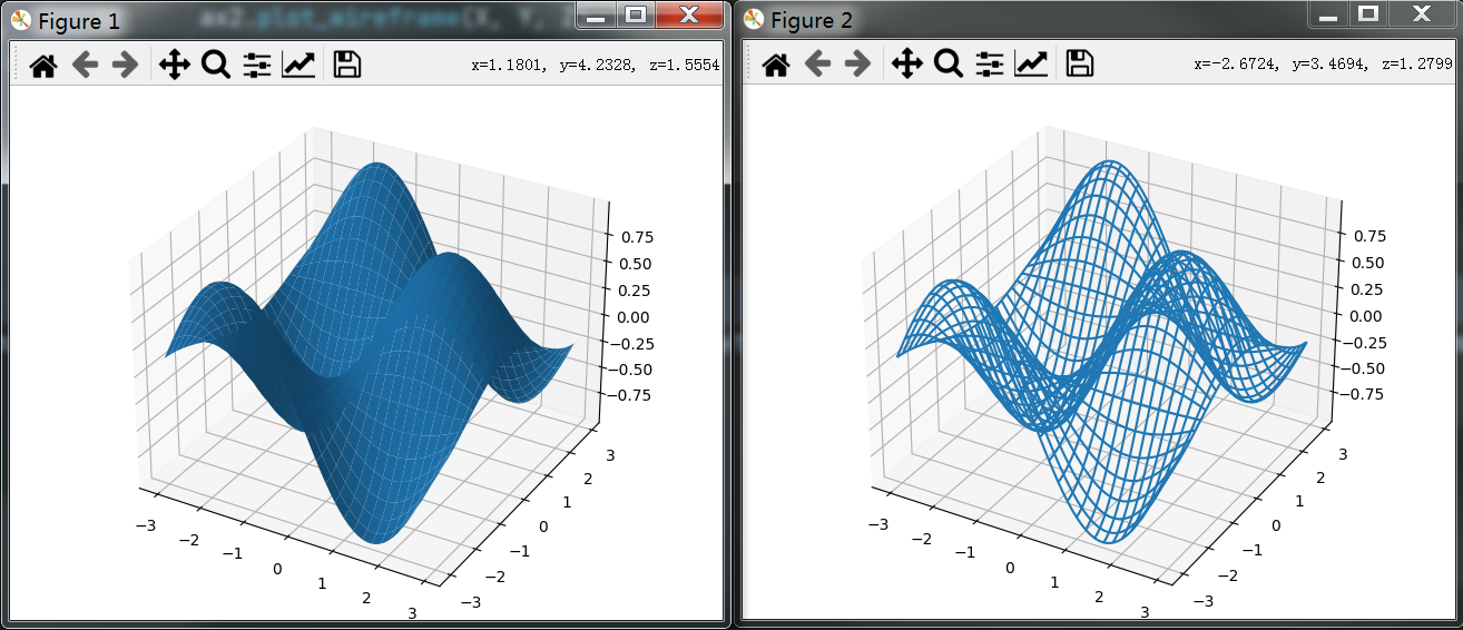
plot_surface(X, Y, Z) 绘制曲面
plot_wireframe(X, Y, Z, color = 'r') 绘制3D线框

上面两个方法X, Y, Z都必须是2D array。

两个方法效果分别如下图
（左边是plot_surface绘制曲面，右边是plot_wireframe绘制线框）

set_xlabel(xlabel)
set_ylabel(ylabel)
set_zlabel(zlabel)

分别设置x，y，z轴的标签

3 Simple3Dplot 绘制效果

import matplotlib.pylab  as p  # Simple3Dplot.py                                   
from mpl_toolkits.mplot3d import Axes3D

print("Please be patient while I do importing & plotting")
delta = 0.1
x = p.arange( -3., 3., delta )
y = p.arange( -3., 3., delta )
X, Y = p.meshgrid(x, y)
Z = p.sin(X) * p.cos(Y)                       # Surface height


fig = p.figure()                               # Create figure
ax = Axes3D(fig)                                  # Plots axes
ax.plot_surface(X, Y, Z)                            # Surface
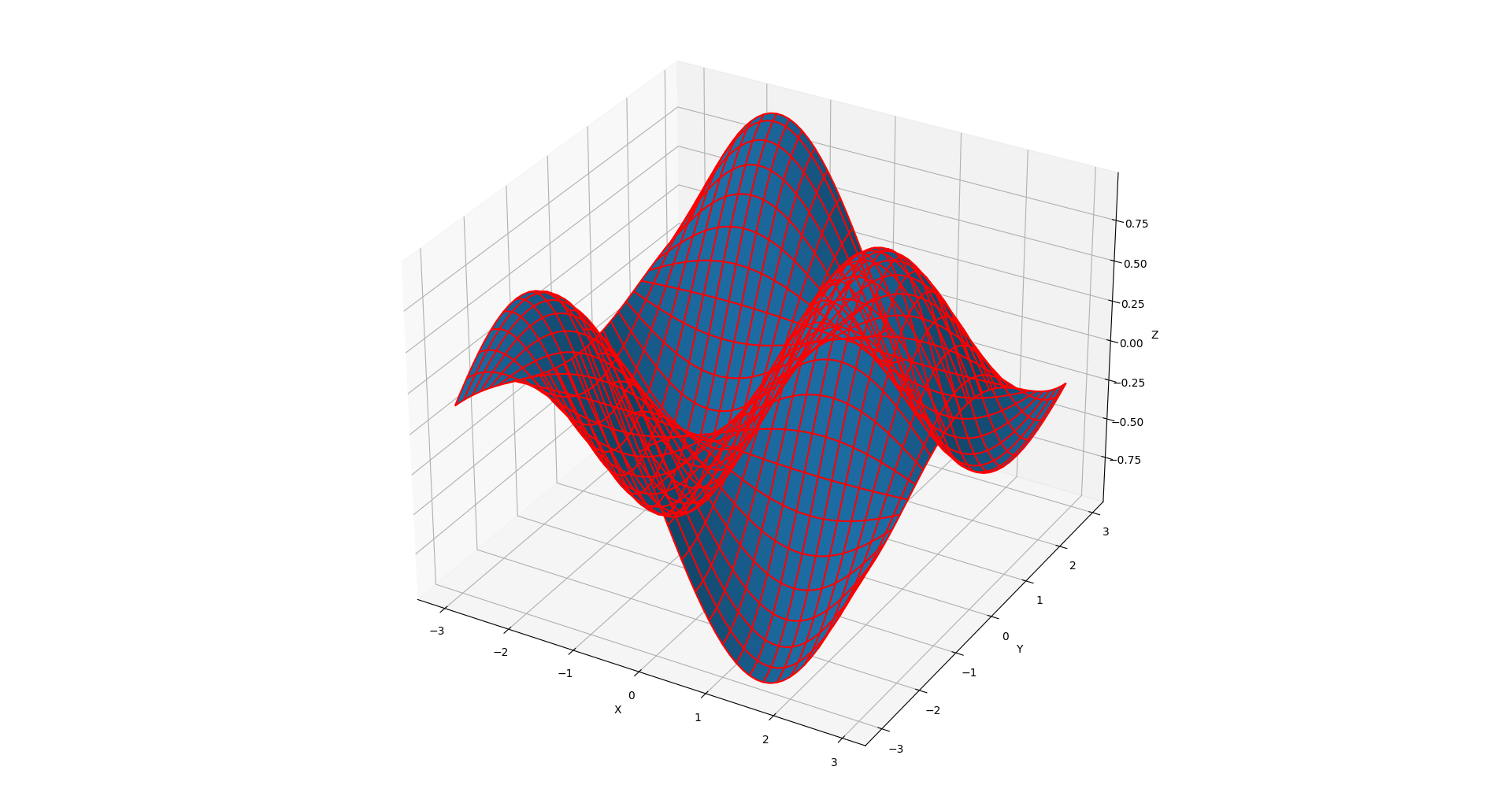
ax.plot_wireframe(X, Y, Z, color = 'r')        # Add wireframe
ax.set_xlabel('X')
ax.set_ylabel('Y')
ax.set_zlabel('Z')
p.show()                                        # Output figure