


每一段代码后都有跑出来的结果
参考网址 https://pytorch.org/tutorials/beginner/blitz/neural_networks_tutorial.html
1. Neural Networks
1.1 Define the network
class Net(nn.Module):
def __init__(self):
super(Net, self).__init__() # 类继承,py2.7的写法,在3中可以写为super().__init__()
# 1 input image channel, 6 output channels, 3x3 square convolution
# kernel
self.conv1 = nn.Conv2d(1, 6, 3) # 定义第一个卷积核的shape
self.conv2 = nn.Conv2d(6, 16, 3) # 第二个卷积核的shape
# an affine operation: y = Wx + b
self.fc1 = nn.Linear(16 * 6 * 6, 120) # 6*6 from image dimension
self.fc2 = nn.Linear(120, 84)
self.fc3 = nn.Linear(84, 10) # 定义了三个全连接层
def forward(self, x):
# Max pooling over a (2, 2) window
x = F.max_pool2d(F.relu(self.conv1(x)), (2, 2)) # 先对x用conv1进行卷积,再ReLU结果最后用2*2窗口池化
# If the size is a square you can only specify a single number
x = F.max_pool2d(F.relu(self.conv2(x)), 2) # 与第一步相同,窗口如果是正方形可以只写一边的边长
x = x.view(-1, self.num_flat_features(x)) # view相当于Numpy中的reshape,将x reshape为一个一维的向量来输入全连接层
x = F.relu(self.fc1(x)) # 全连接层
x = F.relu(self.fc2(x)) # 全连接层
x = self.fc3(x) # 全连接层
return x
def num_flat_features(self, x): # 扁平化向量x
size = x.size()[1:] # all dimensions except the batch dimension
num_features = 1
for s in size:
num_features *= s
return num_features # 返回x除第一个维度以外所有维度的乘积,用于压扁x
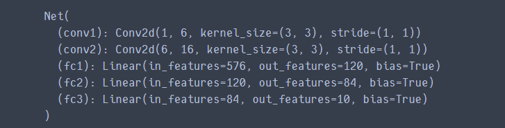
net = Net()
print(net)
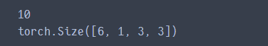
params = list(net.parameters()) # 网络参数列表,一共有十组参数
#print(params)
print(len(params)) # 参数列表长度
print(params[0].size())  # conv1's .weight
input = torch.randn(1, 1, 32, 32) # 生成一个随机张量,1,1,32,32代表num为1,channel为1,高和宽均为32
out = net(input) # 在网络中进行前向传播
print(out)

net.zero_grad() # 将所有参数的梯度缓冲区都置0
out.backward(torch.randn(1, 10)) # 给out一个梯度输入,让梯度进行反向传播
这里没有结果输出,但有一个NOTE
torch.nn only supports mini-batches. The entire torch.nn package only supports inputs that are a mini-batch of samples, and not a single sample.
For example, nn.Conv2d will take in a 4D Tensor of nSamples x nChannels x Height x Width.
If you have a single sample, just use input.unsqueeze(0) to add a fake batch dimension.
1.2 Loss Function
output = net(input) # 前向传播产生一个结果
target = torch.randn(10)  # a dummy target, for example
target = target.view(1, -1)  # make it the same shape as output
criterion = nn.MSELoss() # 误差为MSELoss,也就是均方误差

loss = criterion(output, target) # 求取输出和目标结果之间的均方误差
print(loss)

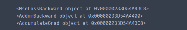
print(loss.grad_fn)  # MSELoss
print(loss.grad_fn.next_functions[0][0])  # Linear,MSELoss的上一级
print(loss.grad_fn.next_functions[0][0].next_functions[0][0])  # ReLU,Linear的上一级
1.3 Backprop
要反向传播误差,我们要做的就是调用loss.backward()。不过,需要清除现存的梯度值,否则梯度将累积到现有的梯度中。
net.zero_grad() # zeroes the gradient buffers of all parameters
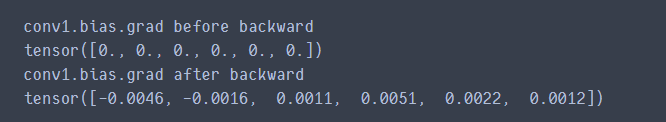
print('conv1.bias.grad before backward')
print(net.conv1.bias.grad) # 梯度置0后的偏置梯度
loss.backward()
print('conv1.bias.grad after backward')
print(net.conv1.bias.grad) # 求取梯度后的偏置梯度值
1.4 Update the weights
在SGD中使用的最简单的更新规则为:
weight = weight - learning_rate * gradient
用python代码实现如下
learning_rate = 0.01
for f in net.parameters():
    f.data.sub_(f.grad.data * learning_rate) # sub_应该是对f.data做减法并且更新到f.data中
import torch.optim as optim # 导入优化器,我们可以采用更多的梯度更新规则,例如Nesterov-SGD,Adam,RMSProp等等

# create your optimizer
optimizer = optim.SGD(net.parameters(), lr=0.01) # 创建一个优化器,采用SGD方法,学习率为0.01

# in your training loop:
optimizer.zero_grad()   # zero the gradient buffers
output = net(input) # 前向传播
loss = criterion(output, target) # 求出误差
loss.backward() # 反向传播
optimizer.step()    # Does the update 使用定义的优化器规则进行参数的更新
2. Trainning a classifier
2.1 Loading and normalizing CIFAR10
这部分要CIFAR10数据集,懒得弄了,就不跑了,只写一下程序注释。
### torchvision是一个图像操作的库
### transforms是对图像做预处理的包
import torch
import torchvision
import torchvision.transforms as transforms

# 预处理
transform = transforms.Compose(
    [transforms.ToTensor(), # PIL图像转化为torch.Tensor
     transforms.Normalize((0.5, 0.5, 0.5), (0.5, 0.5, 0.5))]) # 对张量进行Normalization,此处因为
     #ToTensor操作已把数据处理成了[0,1],那么image-0.5/0.5的范围就是[-1,1]

# 训练集,download=True表示如果本地没有数据集就去INTERNET上下载下来,并对训练集做上述transform的预处理
trainset = torchvision.datasets.CIFAR10(root='./data', train=True,
                                        download=True, transform=transform)

# 加载训练集,batch_size为4,并在每一个epoch中打乱数据,num_workers使用多进程加载的进程数,0代表不使用
trainloader = torch.utils.data.DataLoader(trainset, batch_size=4,
                                          shuffle=True, num_workers=2)

# 测试集,与训练集不一样的地方就是参数train=False
testset = torchvision.datasets.CIFAR10(root='./data', train=False,
                                       download=True, transform=transform)

# 加载测试集,测试集数据不需要打乱
testloader = torch.utils.data.DataLoader(testset, batch_size=4,
                                         shuffle=False, num_workers=2)

# 设置类别元组
classes = ('plane', 'car', 'bird', 'cat', 'deer', 'dog', 'frog', 'horse', 'ship', 'truck')
加载一些数据看看效果:
import matplotlib.pyplot as plt
import numpy as np

# functions to show an image


def imshow(img):
    img = img / 2 + 0.5     # unnormalize 还原图像
    npimg = img.numpy()
    plt.imshow(np.transpose(npimg, (1, 2, 0))) # 改变通道顺序
    plt.show()


# get some random training images
dataiter = iter(trainloader) # 每次迭代取一个Batch,这也就是为何显示四张图片
images, labels = dataiter.next()

# show images
imshow(torchvision.utils.make_grid(images)) # make_grid将多幅图像合并成网格
# print labels
print(' '.join('%5s' % classes[labels[j]] for j in range(4)))
2.2 Define a Convolutional Neural Network
import torch.nn as nn
import torch.nn.functional as F

# 定义一个网络,继承于nn.Module,网络结构为
# Conv1->ReLU->pool->Conv2->ReLU->pool->fc1->fc2->f3->scores
class Net(nn.Module):
    def __init__(self):
        super(Net, self).__init__()
        self.conv1 = nn.Conv2d(3, 6, 5)
        self.pool = nn.MaxPool2d(2, 2)
        self.conv2 = nn.Conv2d(6, 16, 5)
        self.fc1 = nn.Linear(16 * 5 * 5, 120)
        self.fc2 = nn.Linear(120, 84)
        self.fc3 = nn.Linear(84, 10)

    def forward(self, x):
        x = self.pool(F.relu(self.conv1(x)))
        x = self.pool(F.relu(self.conv2(x)))
        x = x.view(-1, 16 * 5 * 5)
        x = F.relu(self.fc1(x))
        x = F.relu(self.fc2(x))
        x = self.fc3(x)
        return x

# 实例化一个网络net
net = Net()
2.3 Define a Loss function and optimizer
import torch.optim as optim

criterion = nn.CrossEntropyLoss() # 交叉熵损失函数
optimizer = optim.SGD(net.parameters(), lr=0.001, momentum=0.9) # 优化器选择带动量的SGD,学习率0.001
2.4 Train the network
for epoch in range(2):  # loop over the dataset multiple times 跑两个epoch

    running_loss = 0.0
    for i, data in enumerate(trainloader, 0): # 从下标为0的地方开始遍历
        # get the inputs; data is a list of [inputs, labels]
        inputs, labels = data

        # zero the parameter gradients
        optimizer.zero_grad() # 清空梯度缓冲区

        # forward + backward + optimize
        outputs = net(inputs) # 前向传播得到scores
        loss = criterion(outputs, labels) # 求出scores的交叉熵损失
        loss.backward() # 进行反向传播求导
        optimizer.step() # 用上面定义的带有动量的SGD优化器进行参数更新

        # print statistics
        running_loss += loss.item() # 累积两千次的Loss
        if i % 2000 == 1999:    # print every 2000 mini-batches
            print('[%d, %5d] loss: %.3f' %
                  (epoch + 1, i + 1, running_loss / 2000))
            running_loss = 0.0 # loss置零,求下一个2000次

print('Finished Training')
保存网络:
PATH = './cifar_net.pth'
torch.save(net.state_dict(), PATH)
2.5 Test the network on the test data
# 这里只是随便从测试集中取几张图片看一下
dataiter = iter(testloader)
images, labels = dataiter.next()

# print images
imshow(torchvision.utils.make_grid(images))
print('GroundTruth: ', ' '.join('%5s' % classes[labels[j]] for j in range(4)))
导入训练好的网络:
net = Net()
net.load_state_dict(torch.load(PATH))
前向传播:
outputs = net(images)
根据前向传播的结果预测类别:
_, predicted = torch.max(outputs, 1) # 选择计算出的outputs中的最大值,第二个参数为dim,1代表行方向的最大值

print('Predicted: ', ' '.join('%5s' % classes[predicted[j]]
                              for j in range(4)))
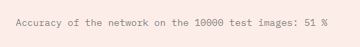
看看在整个测试集上的效果:
correct = 0
total = 0
with torch.no_grad(): # 这次计算不用求梯度,省去一些开销
    for data in testloader:
        images, labels = data
        outputs = net(images)
        _, predicted = torch.max(outputs.data, 1)
        total += labels.size(0) # 总数
        correct += (predicted == labels).sum().item() # 分类正确的数目

print('Accuracy of the network on the 10000 test images: %d %%' % (
    100 * correct / total))
官方训练的结果,好像还行,有一半的正确率:
2.6 Training on GPU
想要在GPU加速训练,可以用如下代码:
device = torch.device("cuda:0" if torch.cuda.is_available() else "cpu")

net.to(device)

# 记得把数据集和标签都放到GPU上去
inputs, labels = data[0].to(device), data[1].to(device)


 8500
8500

 被折叠的 条评论
为什么被折叠?
被折叠的 条评论
为什么被折叠?
 到【灌水乐园】发言


