卡尔曼滤波笔记+C代码实现

musanruqiu

已于 2024-08-12 09:38:21 修改

阅读量7.7k

点赞数 9

分类专栏：算法文章标签： c语言

于 2022-09-24 17:52:28 首次发布

本文链接：https://blog.youkuaiyun.com/musanruqiu/article/details/126994167

版权

算法专栏收录该内容

4 篇文章

订阅专栏

一、前言

学习视频来自B站up主 DR_CAN的卡尔滤波器的讲解。

二、递归算法

估计真实数据（求平均值）

A = 1/k * (Z1 + Z2 + Z3 + ......+ Zk )

= 1/k * (Z1 + Z2 + Z3 + ......+ Z(k-1)) + 1/k * Zk

= 1/k * (k -1)/ (k-1) * (Z1 + Z2 + Z3 + ......+ Z(k-1)) + 1/k * Zk

= (k-1)/k * A(k-1) + 1/k * Zk

= A(k-1) - 1/k * A(k-1) + 1/k * Zk

A = A(k-1) + 1/k * (Zk - A(k-1))

1/k 可以用 Kk 代替。

公式描述为：

当前估计值 = 上一次估计值 + 系数 * （当前测量值 - 上一次估计值）

A :当前估计值 A（k-1）:上一次估计值 1/k (或Kk) : 系数（也称卡尔曼增益）

Zk : 当前测量值 Z（k-1）: 上一次测量值

求Kk

Kk = Eest(k-1) / ( Eest(k-1) + Emea(k))

Eest(k-1) : 上一次估计误差

Emea(k) ：当前测量误差

由公式可见：当估计误差远大于测量误差时 Kk 趋近于 1，当前估计值趋近于当前的测量值

当估计误差远小于测量误差时 Kk 趋近于 0，当前估计值趋近于上一次估计值

求估计误差

Eest(k) = （1 - Kk）* Eest(k-1) //不作推导

C代码实现

执行顺序为：

STEP1 ：计算Kk;

STEP 2 : 计算A；

STEP 2 : 计算Eest(k)；

假设一个物体真实长度为50，测量工具的误差为3，第0次的估计值为40，第0次的估计误差为5，当前测量的值为51。代码实现如下：

#include <stdio.h>
#include <math.h>
#include <stdlib.h>
#include <string.h>

#define         ERR_MEA      3
#define         ACTUAL_VAL   50
typedef struct{
    float ERR_est_last;                 //估计误差
    float ERR_mea;                      //测量误差
    float VAL_est_last;                 //上一次估计值
    float VAL_est_curr;                 //当前估计值    
    float VAL_mea_curr;                 //当前测量值
    float Kk;                           //卡尔曼增益
} KALMAN_PARM;

KALMAN_PARM kalman_val;
void CAL_VALUE_CURRENT(KALMAN_PARM *val);
int main(void){
    memset(&kalman_val, 0,sizeof(KALMAN_PARM));
    kalman_val.ERR_mea          =  ERR_MEA;                      //假设测量误差始终为3          
    kalman_val.ERR_est_last     =  5.0;                          //给定一个初始估计误差
    kalman_val.VAL_est_last     =  40;                           //给定一个初始估计值
    kalman_val.VAL_mea_curr     =  51;                           //给定一个当前的测量值
    for(int i = 0; i < 1000; i++){
        CAL_VALUE_CURRENT(&kalman_val);
    }
    return 0;
}
//计算当前估计值
void CAL_VALUE_CURRENT(KALMAN_PARM *val){
    val->VAL_mea_curr = ACTUAL_VAL + rand()%3;                                                  //制造一个在实际值上下浮动的测量值
    val->Kk           = val->ERR_est_last / (val->ERR_est_last + val->ERR_mea);                 //计算卡尔曼增益
    val->VAL_est_curr = val->VAL_est_last + val->Kk * (val->VAL_mea_curr - val->VAL_est_last);  //计算当前估计值
    val->VAL_est_last = val->VAL_est_curr;
    val->ERR_est_last = (1.0 - val->Kk) * val->ERR_est_last;                                    //更新估计误差
    printf("当前估计值为：%f\n", val->VAL_est_curr);
}

以上的做法是基于一个测量工具对一个事物的多次测量，估计结果只于上一次的估计值与当前的测量值相关。

二、数据融合

假设有两个称去称一个物体，第一个称的（Z1）30，第二个称得（Z2）32。且第一个称的标准差为(B1)2，第二个的标准差为(B2)4。测量结果满足正态分布。

A (两组数据的最优解) = Z1 + K * （Z2 -Z1）, 设X为A的标准差

X的平方 = VAR( Z1 + K * （Z2 -Z1)) // VAR 代表方差

= VAR( Z1 - K*Z1 + K * Z2)

= VAR((1- K)*Z1 + K * Z2 )

= (1- K) * (1- K) * VAR(Z1) + K * K * (Z2)

= (1- K) * (1- K) * B1*B1 + K * K * B2*B2

对K求导令其等于0

-2（1-K）* B1*B1 + 2 *K *B2 * B2 = 0

K = （B1*B1）/ ((B1*B1) + (B2*B2 )) = 0.2

结合上述可 A= 30 + 0.2*(32 - 30) = 30.4

X的平方 = (1-0.2)的平方 * 2的平方 + 0.2的平方 * 4的平方 = 3.2

X = 1.79

c代码实现：

#include <stdio.h>
#include <math.h>
#include <string.h>

typedef struct{
    double val;                  //测量值
    double devi;                 //标准差
} Normal_distribution;

Normal_distribution  Mea1,Mea2;                    //定义两个正太分布值
double optimal_solution;                            //最优解   
double new_devi;                                 //最优解的标准差    
double  Kk;                                        
//数据融合
void Data_Fusion(Normal_distribution data1,  Normal_distribution data2){
    Kk = pow(2.0, data1.devi) / (pow(2.0, data1.devi) + pow(2.0, data2.devi));
    printf("卡尔曼增益为：%f\n", Kk);    
    optimal_solution = data1.val + Kk * (data2.val - data1.val);
    printf("最优解为：%f\n", optimal_solution);
}

void UPdata_devi(Normal_distribution data1,  Normal_distribution data2){
//    new_devi = (pow(2.0 , (1.0 - Kk)) * pow(2.0, data1.devi))  + (pow(2.0, Kk) * pow(2.0, data2.devi));
    new_devi = (1.0 - Kk) * (1.0 - Kk) * data1.devi * data1.devi +  Kk*Kk * data2.devi*data2.devi;
    new_devi = sqrt(new_devi);
    printf("最优解的标准差为：%f\n", new_devi);
}

int main(void){
    memset(&Mea1, 0,sizeof(Mea1));
    memset(&Mea2, 0,sizeof(Mea2));
    
    Mea1.val   = 30;                  //先给定两个初始值
    Mea1.devi  = 2;
    Mea2.val   = 32;
    Mea2.devi  = 4;
    Data_Fusion(Mea1,Mea2);
    UPdata_devi(Mea1,Mea2);
    return 0;
}

上述方法为寻求两种测量工具对同一物体测量结果的最优解。

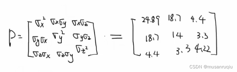
三、协方差矩阵

方差与协方差在一个矩阵中表现出来，主要是体现不同变量之间的关联性。

假设有以下样本：

	身高/X	体重/Y	年龄/z
A	179	74	33
B	187	80	31
C	175	71	28
AVG	180.5	75	30.7

VAR(X) = 24.89 协方差（XY） = 18.7

VAR(Y) = 14 协方差（XZ） = 18.7

VAR(Z) = 4.22 协方差（YZ） = 18.7

则矩阵表示如下：

引用上述样本，C代码实现如下：

#include <stdio.h>
#include <math.h>
#include <stdlib.h>

double Covariance_Matrix[9] ;
typedef struct{
    double Height;
    double Weight;
    double Age;
} SAMPIE;
SAMPIE p1 = {179,74,33};
SAMPIE p2 = {187,80,31};
SAMPIE p3 = {175,71,28};

//构建矩阵
void COV_MAT_CAL(void){
    double avg_X, avg_Y,avg_Z;                                          //三个平均值  分别对应Height，Weight，Age
    double COV_X_2, COV_Y_2, COV_Z_2, COV_X_Y,COV_X_Z, COV_Y_Z;         //6个协方差的值
    avg_X  = (p1.Height + p2.Height + p3.Height) / 3.0;
    avg_Y  = (p1.Weight + p2.Weight + p3.Weight) / 3.0;
    avg_Z  = (p1.Age    + p2.Age    + p3.Age)    / 3.0;

    COV_X_2 = ((p1.Height - avg_X) * (p1.Height - avg_X) + (p2.Height - avg_X) * (p2.Height - avg_X) + (p3.Height - avg_X) * (p3.Height - avg_X)) / 3.0;
    COV_Y_2 = ((p1.Weight - avg_Y) * (p1.Weight - avg_Y) + (p2.Weight - avg_Y) * (p2.Weight - avg_Y) + (p3.Weight - avg_Y) * (p3.Weight - avg_Y)) / 3.0;
    COV_Z_2 = ((p1.Age - avg_Z)*(p1.Age - avg_Z) + (p2.Age - avg_Z)*(p2.Age - avg_Z) + (p3.Age - avg_Z)*(p3.Age - avg_Z))/3.0;
    COV_X_Y = ((p1.Height - avg_X) * (p1.Weight - avg_Y) + (p2.Height - avg_X) * (p2.Weight - avg_Y) + (p3.Height - avg_X) * (p3.Weight - avg_Y)) / 3.0;
    COV_X_Z = ((p1.Height - avg_X) * (p1.Age - avg_Z) + (p2.Height - avg_X) * (p2.Age - avg_Z) + (p3.Height - avg_X) * (p3.Age - avg_Z)) / 3.0;
    COV_Y_Z = ((p1.Weight - avg_Y) * (p1.Age - avg_Z) + (p2.Weight - avg_Y) * (p2.Age - avg_Z) + (p3.Weight - avg_Y) * (p3.Age - avg_Z)) / 3.0;

    Covariance_Matrix[0] = COV_X_2;
    Covariance_Matrix[1] = COV_X_Y;
    Covariance_Matrix[2] = COV_X_Z;
    Covariance_Matrix[3] = COV_X_Y;
    Covariance_Matrix[4] = COV_Y_2;
    Covariance_Matrix[5] = COV_Y_Z;
    Covariance_Matrix[6] = COV_X_Z;
    Covariance_Matrix[7] = COV_Y_Z;
    Covariance_Matrix[8] = COV_Z_2;

    printf("%f  %f  %f\n%f  %f  %f\n%f  %f  %f\n", Covariance_Matrix[0],Covariance_Matrix[1],Covariance_Matrix[2],\
                                                   Covariance_Matrix[3],Covariance_Matrix[4],Covariance_Matrix[5],\
                                                   Covariance_Matrix[6],Covariance_Matrix[7],Covariance_Matrix[8] );
}



int main(void){
    COV_MAT_CAL();
    return 0;
}

四、状态空间表达

大抵如下：

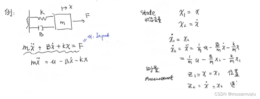
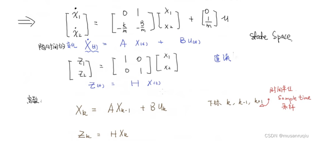
X上的一个点，两个点分别为对时间的一阶求导和二阶求导。

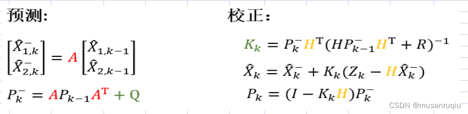
五、视频中，二阶卡尔曼滤波器的C实现

矩阵的运算包括加、减、乘、数乘、转置、行列式、逆矩阵、代数余子式。

数据来源视频中提供的excel表。自行获取。

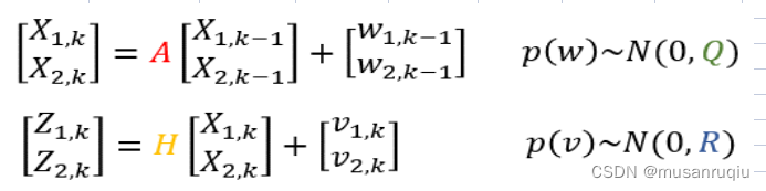
C代码如下：

#include <stdio.h>
#include <math.h>
#include <stdlib.h>

typedef struct{
    double A11;
    double A12;
    double A21;
    double A22;
} TWO_DIM_Matrix;                      //定义2x2的矩阵

typedef struct{
    double Position;                   //位置
    double Velocity;                   //速度
}Statue;

typedef struct{
    double W1;                        //状态位置误差
    double W2;                        //状态速度误差
}Statue_ERR;

typedef struct{
    double V1;                        //测量位置误差
    double V2;                        //测量速度误差
}MEA_ERR;

//状态位置过程误差
double E1[30] = { 0.097,  0.150,  0.108,  -0.293,  0.214, -0.024, -0.097, -0.414, -0.466, -0.287,\
                  0.316, -0.165,  0.222,   0.314, -0.532, -0.083, -0.144, -0.305, -0.499, -0.194,\
                  0.177, -0.310, -0.446,  -0.024,  0.239,  0.353, -0.026, -0.621,  0.167,  0.164};
//状态速度过程误差
double E2[30] = { 0.159, -0.418,  0.044,  -0.115, -0.375, -0.165, -0.390, -0.162,  0.061, -0.024,\
                 -0.309,  0.060,  0.201,   0.303, -0.305, -0.325,  0.227,  0.176, -0.182,  0.265,\
                 -0.179,  0.140,  0.051,  -0.761,  0.146, -0.030,  0.340,  0.399, -0.421, -0.473};
//测量位置过程误差
double E3[30] = {-0.208,  0.911, -0.899,  -0.232, -0.114,  0.399, -0.493,  0.400,  0.208, -0.878,\
                  1.933,  0.161, -1.906,  -1.473,  0.417, -0.744, -0.576, -1.120,  0.838, -1.633,\
                 -0.261, -0.214, -0.026,   0.015,  0.230,  1.321,  1.287, -1.508, -1.194,  1.420};
//测量速度过程误差 
double E4[30] = { 0.272,  0.414,  0.438,  -0.985, -0.183, -0.382,  1.181, -0.731, -0.235, -0.639,\
                  1.352,  1.352,  1.187,  -0.200,  1.082,  1.364,  0.180, -0.610, -0.443,  0.301,\
                  0.041,  0.165, -0.164,   0.399, -0.923, -0.613,  0.131,  0.475,  0.428, -0.185};    

Statue_ERR        Process_Err[30];                                 //过程误差
MEA_ERR           measure_Err[30];                                 //测量误差
Statue            X[30], Z[30], X_Hat[30], X_Hat_PRE[30];              //
TWO_DIM_Matrix    Q, R, A, H, E, P_k[30], P_k_PRE[30],K_k[30];

void Status_Param_init(void){
    for(int i = 0; i<30;i++){                             //将样本误差数据存入数组
        Process_Err[i].W1 = E1[i];
        Process_Err[i].W2 = E2[i];
    }
    X[0].Position = 0.0;                                  //给定初始位置和速度值
    X[0].Velocity = 1.0;

    for(int j = 1 ; j<30; j++){
        X[j].Position = A.A11*X[j-1].Position + A.A12*X[j-1].Velocity + Process_Err[j-1].W1;
        X[j].Velocity = A.A22*X[j-1].Velocity + Process_Err[j-1].W2;                              //A.A21  的值为0  可以不写
//        printf("%f\n",X[j].Velocity); 
    }
}

void Mea_Param_init(void){
    for(int i = 0; i<30; i++){
        measure_Err[i].V1 = E3[i];
        measure_Err[i].V2 = E4[i];
    }

    for(int j =1; j<30; j++){
        Z[j].Position = H.A11*X[j].Position + H.A12*X[j-1].Velocity + measure_Err[j].V1;
        Z[j].Velocity = H.A22*X[j].Velocity + measure_Err[j].V2;                               //A.A21 的值为0   可以不写
//        printf("%f\n",Z[j].Velocity); 
    }
}

void TWO_DIM_Matrix_PARAM_init(void){
    //Q Matrix init
    Q.A11 = 0.1;    Q.A12 = 0.0;
    Q.A21 = 0.0;    Q.A22 = 0.1;
   //R Matrix init
    R.A11 = 1.0;    R.A12 = 0.0;
    R.A21 = 0.0;    R.A22 = 1.0;
    //A Matrix init
    A.A11 = 1.0;    A.A12 = 1.0;
    A.A21 = 0.0;    A.A22 = 1.0;
    //H Matrix init
    H.A11 = 1.0;    H.A12 = 0.0;
    H.A21 = 0.0;    H.A22 = 1.0;
    //E Matrix init
    E.A11 = 1.0;    E.A12 = 0.0;
    E.A21 = 0.0;    E.A22 = 1.0;

    P_k[0].A11 = 1.0;   P_k[0].A12 = 0.0;
    P_k[0].A21 = 0.0;   P_k[0].A22 = 1.0;
}
//矩阵的转置运算
TWO_DIM_Matrix Matrix_Transpose(TWO_DIM_Matrix input_matrix){
    TWO_DIM_Matrix Result;
    Result.A11 = input_matrix.A11;
    Result.A12 = input_matrix.A21;
    Result.A21 = input_matrix.A12;
    Result.A22 = input_matrix.A22;
    return Result;
}
//矩阵的代数余子式
TWO_DIM_Matrix Matrix_Congruent(TWO_DIM_Matrix input_matrix){
    TWO_DIM_Matrix Result;
    Result.A11 = input_matrix.A22;
    Result.A12 = input_matrix.A21*(-1);
    Result.A21 = input_matrix.A12*(-1);
    Result.A22 = input_matrix.A11; 
    return Result;
}
//矩阵相乘
TWO_DIM_Matrix Matrix_Multi(TWO_DIM_Matrix input_matrix1 , TWO_DIM_Matrix input_matrix2){
    TWO_DIM_Matrix Result;
    Result.A11 = input_matrix1.A11*input_matrix2.A11 + input_matrix1.A12*input_matrix2.A21;
    Result.A12 = input_matrix1.A11*input_matrix2.A12 + input_matrix1.A12*input_matrix2.A22;
    Result.A21 = input_matrix1.A21*input_matrix2.A11 + input_matrix1.A22*input_matrix2.A21;
    Result.A22 = input_matrix1.A21*input_matrix2.A12 + input_matrix1.A22*input_matrix2.A22;
    return Result;
}
//矩阵相加
TWO_DIM_Matrix Matrix_ADD(TWO_DIM_Matrix input_matrix1 , TWO_DIM_Matrix input_matrix2){
    TWO_DIM_Matrix Result;
    Result.A11 = input_matrix1.A11 + input_matrix2.A11;
    Result.A12 = input_matrix1.A12 + input_matrix2.A12;
    Result.A21 = input_matrix1.A21 + input_matrix2.A21;
    Result.A22 = input_matrix1.A22 + input_matrix2.A22;
    return Result;
}

//矩阵相减
TWO_DIM_Matrix Matrix_Reduce(TWO_DIM_Matrix input_matrix1 , TWO_DIM_Matrix input_matrix2){
    TWO_DIM_Matrix Result;
    Result.A11 = input_matrix1.A11 - input_matrix2.A11;
    Result.A12 = input_matrix1.A12 - input_matrix2.A12;
    Result.A21 = input_matrix1.A21 - input_matrix2.A21;
    Result.A22 = input_matrix1.A22 - input_matrix2.A22;
    return Result;
}
//矩阵的逆矩阵
TWO_DIM_Matrix Inverse_Matrix(TWO_DIM_Matrix input_matrix){
    TWO_DIM_Matrix Result;
    double A;
    A = input_matrix.A11*input_matrix.A22 - input_matrix.A12*input_matrix.A21;
    A = 1.0/A;  
    Result = Matrix_Congruent(input_matrix);
    Result.A11 = A * Result.A11;
    Result.A12 = A * Result.A12;
    Result.A21 = A * Result.A21;
    Result.A22 = A * Result.A22; 
    return Result;
}

void Kalman_Calc(void){
    TWO_DIM_Matrix buffer;
    X_Hat[0].Position = 0.0;
    X_Hat[0].Velocity = 1.0;
    for(int i = 1 ; i<30; i++){
        X_Hat_PRE[i].Position = A.A11 * X_Hat[i-1].Position + A.A12*X_Hat[i-1].Velocity;
        X_Hat_PRE[i].Velocity = A.A22 * X_Hat[i-1].Velocity;
        buffer = Matrix_Multi(A, P_k[i-1]);
        buffer = Matrix_Multi(buffer, Matrix_Transpose(A));
        P_k_PRE[i] = Matrix_ADD(buffer, Q);
        buffer = Matrix_ADD(P_k_PRE[i], R);
        buffer = Inverse_Matrix(buffer);
        K_k[i] = Matrix_Multi(P_k_PRE[i], buffer);
        X_Hat[i].Position = X_Hat_PRE[i].Position + K_k[i].A11 * (Z[i].Position - X_Hat_PRE[i].Position) + K_k[i].A12 * (Z[i].Velocity - X_Hat_PRE[i].Velocity);
        X_Hat[i].Velocity = X_Hat_PRE[i].Velocity + K_k[i].A21 * (Z[i].Position - X_Hat_PRE[i].Position) + K_k[i].A22 * (Z[i].Velocity - X_Hat_PRE[i].Velocity);
        P_k[i] = Matrix_Multi(Matrix_Reduce(E,K_k[i]), P_k_PRE[i]);
    }

}
int main(void){
    int i;
    TWO_DIM_Matrix_PARAM_init();
    Status_Param_init();
    Mea_Param_init();
    Kalman_Calc();
    for(i = 0;i<30;i++){
        printf("%f\n",X_Hat_PRE[i].Velocity);
    }
    for(i = 0;i<30;i++){
        printf("%f\n",X_Hat[i].Velocity);
    }
    return 0;
}