卡尔曼滤波实例分析（三）——待续

1 问题

之前的案例都是线线性的，但实际情况常面临很多非线性问题，比如：
假设平面上有一飞行器，初始坐标为$(x_0,y_0)$，需要该飞行器基于该平面完成一个圆形运动，模型如下；
（1）建模
$x_{t+1}=x_t+v_x\ast dt\ast cos(w)$
$y_{t+1}=y_t+v_y\ast dt\ast sin(w)$
$w_{t+1}=w_t+\Delta (w)\ast dt$

import numpy as np
import matplotlib.pyplot as plt
"""
速度：X = X0 + V_X * t * cos(w)
位置：Y = Y0 + V_Y * t * sin(w)
角速度：W = W0 + Dw * t

"""
DT = 0.1
SIM_TIME = 500.0  

H = np.array([[1.0, 0.0],
              [0.0, 1.0]])



def calc_input():
    v = 1.0  # [m/s]
    yawrate = 0.1  # [rad/s]
    u = np.array([[v], [yawrate]])
    return u

def motion_model(x,u):
    
    A = np.array([[1.0, 0.0,0.0],
                  [0.0, 1.0,0.0],
                  [0.0, 0.0,1.0]])
    
    B = np.array([[DT * np.cos(x[2, 0]), 0],
                  [DT * np.sin(x[2, 0]), 0],
                  [0.0, DT]])
    
    x = A @ x +B @ u
    return x
   
def observation_model(x):
    H = np.array([
        [1, 0, 0],
        [0, 1, 0]])

    z = H @ x
    return z
    
time=0

x_array = []    
y_array = []

xTrue = np.zeros((3, 1))
u = np.array([[1. ],
       [0.01]])
    
while SIM_TIME >= time:
   
    xTrue = motion_model(xTrue,u)
    x_array.append(xTrue[0,0])
    y_array.append(xTrue[1,0])
    time += DT
    
plt.figure(0)     
plt.plot(x_array,y_array,'g')
plt.show() 

然而现实总存在各种噪声，以至于模型并不会像设计那样得到想要的结构，在上述模型的输入和观测加入噪声。可以得到观测模型

def observation(x, xd, u):
    x = motion_model(x, u)

    z = observation_model(xTrue) + NOISE_OP @ np.random.randn(2, 1)

    ud = u + NOISE_INPUT @ np.random.randn(2, 1)

    xd = motion_model(xd, ud)

    return x, z, xd, ud

运行后能的到如下结果：

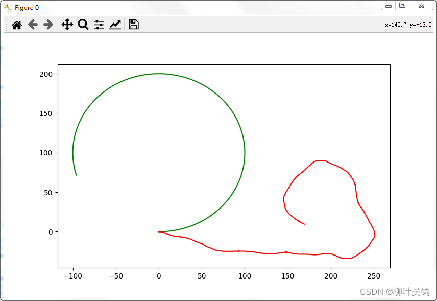
可见失之毫厘谬以千里，如果不加以滤波和修正，该飞行器将不会按理想的运行轨迹运行。
由于所构建的模型引入了三角函数，该模型将不是一个线性模型，卡尔曼滤波将不再适用，因此引入了扩展卡尔曼滤波。
首先需要构建雅克比矩阵：
有模型函数可得：

（2）状态空间方程
略

2 算法实现

3仿真结果