matplotlib部件（widgets）之子图工具（plt.subplot_tool()与Subplottool类）

子图工具Subplottool类概述

matplotlib部件（widgets）提供了子图工具（Subplottool类）用于调整子图的相关参数（边距、间距）。
子图工具实现定义为matplotlib.widgets.Subplottool类，继承关系为：Widget->AxesWidget->Subplottool。
Subplottool类的签名为class matplotlib.widgets.SubplotTool(targetfig, toolfig)。

Subplottool类构造函数的参数为：

• targetfig：子图工具控制的图像，类型为matplotlib.figure.Figure的实例。
• toolfig：子图工具所在的图像，类型为matplotlib.figure.Figure的实例。

子图工具由6个滑动条和1个重置按钮构成。

• Subplottool类通过6个滑动条调整图像子图的边距、间距等参数。Subplottool类通过将targetfig.subplots_adjust()方法与滑动条的on_changed(func)方法绑定实现对图像子图参数的调整。
• Subplottool类的重置按钮回调函数的基本功能其实就是滑动条的reset()方法

plt.subplot_tool()原理

pyplot模块提供了subplot_tool()函数用于快速构造子图工具。

subplot_tool()函数的签名为def subplot_tool(targetfig=None) -> SubplotTool(targetfig, toolfig)
subplot_tool()函数的参数为targetfig，即需要调整子图的图像，类型为matplotlib.figure.Figure的实例，默认值为None。
subplot_tool()函数的返回值为SubplotTool(targetfig, toolfig)。

根据subplot_tool()函数可知，如果targetfig参数为None，那么targetfig = gcf()，即当前图像。subplot_tool()函数随后创建一个没有工具栏的图像toolfig，完成SubplotTool()实例的构造。

案例：官方示例

https://matplotlib.org/gallery/subplots_axes_and_figures/subplot_toolbar.html
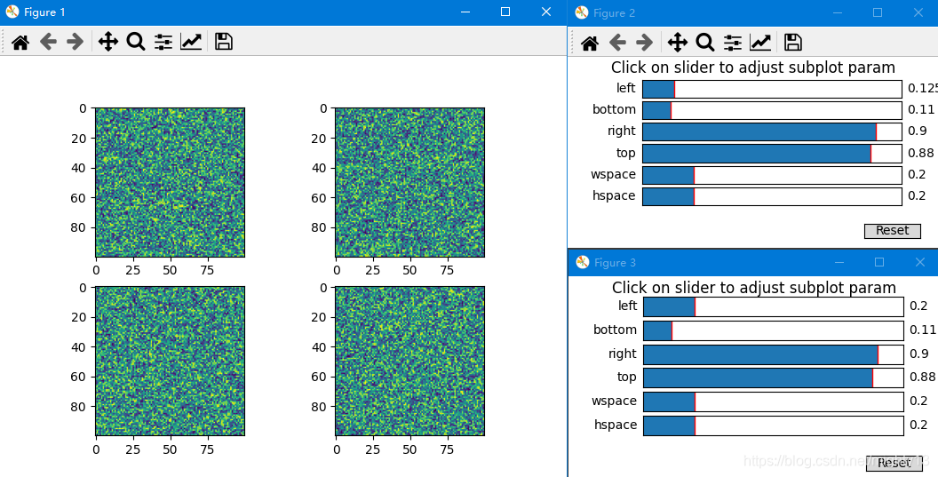
Figure2为直接使用Subplottool类创建的工具，Figure3为使用subplot_tool函数创建的工具。

import matplotlib.pyplot as plt
import numpy as np
from matplotlib.widgets import SubplotTool

np.random.seed(19680801)
fig, axs = plt.subplots(2, 2)
axs[0, 0].imshow(np.random.random((100, 100)))
axs[0, 1].imshow(np.random.random((100, 100)))
axs[1, 0].imshow(np.random.random((100, 100)))
axs[1, 1].imshow(np.random.random((100, 100)))

# 使用SubplotTool类创建工具
fig_tool = plt.figure(figsize=(6, 3))
tool = SubplotTool(fig,fig_tool)
# 使用subplot_tool函数创建工具
plt.subplot_tool()
plt.show()

源码

plt.subplot_tool()源码

 def subplot_tool(targetfig=None):
    """
    Launch a subplot tool window for a figure.

    A :class:`matplotlib.widgets.SubplotTool` instance is returned.
    """
    if targetfig is None:
        targetfig = gcf()

    with rc_context({'toolbar': 'None'}):  # No nav toolbar for the toolfig.
        toolfig = figure(figsize=(6, 3))
    toolfig.subplots_adjust(top=0.9)

    if hasattr(targetfig.canvas, "manager"):  # Restore the current figure.
        _pylab_helpers.Gcf.set_active(targetfig.canvas.manager)

    return SubplotTool(targetfig, toolfig)

Subplottool类部分源码

 self._sliders = []
names = ["left", "bottom", "right", "top", "wspace", "hspace"]
# The last subplot, removed below, keeps space for the "Reset" button.
for name, ax in zip(names, toolfig.subplots(len(names) + 1)):
    ax.set_navigate(False)
    slider = Slider(ax, name,
                    0, 1, getattr(targetfig.subplotpars, name))
    slider.on_changed(self._on_slider_changed)
    self._sliders.append(slider)
    
    
with cbook._setattr_cm(toolfig.subplotpars, validate=False):
    self.buttonreset.on_clicked(self._on_reset)
        
def _on_slider_changed(self, _):
    self.targetfig.subplots_adjust(
        **{slider.label.get_text(): slider.val
            for slider in self._sliders})
    if self.drawon:
        self.targetfig.canvas.draw()

def _on_reset(self, event):
    with ExitStack() as stack:
        # Temporarily disable drawing on self and self's sliders.
        stack.enter_context(cbook._setattr_cm(self, drawon=False))
        for slider in self._sliders:
            stack.enter_context(cbook._setattr_cm(slider, drawon=False))
        # Reset the slider to the initial position.
        for slider in self._sliders:
            slider.reset()
    # Draw the canvas.
    if self.drawon:
        event.canvas.draw()
        self.targetfig.canvas.draw()