倒立摆串行PID算法matlab仿真

以下是一个简单的 倒立摆串行PID 算法的 MATLAB 仿真示例。在这个示例中，我们实现了两个 PID 控制器：一个控制摆杆的角度，另一个控制小车的位置。

1. 系统建模

我们将倒立摆的物理模型简化为一个具有以下方程的动力学系统：

小车的质量为 m1​

摆杆的质量为 m2​

摆杆的长度为 L

小车的位置为 x

摆杆的角度为 θ

倒立摆的动态方程基于拉格朗日方程（简化模型）：

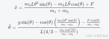
在该模型中，控制力 F 来自 PID 控制器。

2. PID 控制器设计

我们定义两个PID控制器：

PID 控制器1：控制摆杆的角度。

PID 控制器2：控制小车的位置。

3. MATLAB 仿真代码

% MATLAB script for serial PID control of an inverted pendulum

clear;

clc;

% Simulation parameters

dt = 0.01; % Time step

T = 10;    % Total simulation time

steps = T / dt; % Number of steps

time = 0:dt:T-dt; % Time vector

% System parameters

m1 = 1.0; % Mass of the cart (kg)

m2 = 0.2; % Mass of the pendulum (kg)

L = 1.0;  % Length of the pendulum (m)

g = 9.81; % Gravitational acceleration (m/s^2)

% Initial conditions

x = 0;      % Initial cart position (m)

theta = pi/4; % Initial pendulum angle (rad)

x_dot = 0;   % Initial cart velocity (m/s)

theta_dot = 0; % Initial pendulum angular velocity (rad/s)

% PID controller parameters (cart position control)

Kp_x = 10;

Ki_x = 1;

Kd_x = 1;

% PID controller parameters (pendulum angle control)

Kp_theta = 100;

Ki_theta = 10;

Kd_theta = 5;

% Initialize variables for PID

integral_x = 0;

integral_theta = 0;

error_x_prev = 0;

error_theta_prev = 0;

% Store results for plotting

x_vals = zeros(1, steps);

theta_vals = zeros(1, steps);

x_dot_vals = zeros(1, steps);

theta_dot_vals = zeros(1, steps);

% Simulation loop

for i = 1:steps

    % Compute PID for pendulum angle control (θ)

    error_theta = theta; % Set desired θ = 0 (upright position)

    integral_theta = integral_theta + error_theta * dt;

    derivative_theta = (error_theta - error_theta_prev) / dt;

    pid_theta_output = Kp_theta * error_theta + Ki_theta * integral_theta + Kd_theta * derivative_theta;

    error_theta_prev = error_theta;

   

    % Compute PID for cart position control (x)

    error_x = 0 - x; % Set desired x = 0 (center position)

    integral_x = integral_x + error_x * dt;

    derivative_x = (error_x - error_x_prev) / dt;

    pid_x_output = Kp_x * error_x + Ki_x * integral_x + Kd_x * derivative_x;

    error_x_prev = error_x;

   

    % Compute forces acting on the system (F = pid_theta_output + pid_x_output)

    F = pid_theta_output + pid_x_output;

    % Equations of motion (simplified)

    % x_double_dot and theta_double_dot are derived from the system dynamics

    % For simplicity, use simplified models in terms of force and angles.

    denom = m1 + m2 * (1 - cos(theta)^2);

    x_double_dot = (F + m2 * L * theta_dot^2 * sin(theta) - m2 * g * sin(theta) * cos(theta)) / denom;

    theta_double_dot = (g * sin(theta) - cos(theta) * (F + m2 * L * theta_dot^2 * sin(theta))) / (L * (4/3 - (m2 * cos(theta)^2) / (m1 + m2)));

    % Update velocities and positions

    x_dot = x_dot + x_double_dot * dt;

    theta_dot = theta_dot + theta_double_dot * dt;

    x = x + x_dot * dt;

    theta = theta + theta_dot * dt;

    % Store the results for plotting

    x_vals(i) = x;

    theta_vals(i) = theta;

    x_dot_vals(i) = x_dot;

    theta_dot_vals(i) = theta_dot;

end

% Plot results

figure;

subplot(2,1,1);

plot(time, x_vals, 'r', 'LineWidth', 2);

title('Cart Position');

xlabel('Time (s)');

ylabel('Position (m)');

subplot(2,1,2);

plot(time, theta_vals, 'b', 'LineWidth', 2);

title('Pendulum Angle');

xlabel('Time (s)');

ylabel('Angle (rad)');

4. 说明

系统参数：

m1：小车的质量。

m2：摆杆的质量。

L：摆杆的长度。

g：重力加速度。

PID参数：

Kp_x, Ki_x, Kd_x：控制小车位置的PID参数。

Kp_theta, Ki_theta, Kd_theta：控制摆杆角度的PID参数。

状态更新：

小车的加速度和摆杆的角加速度通过方程来计算。这里使用简化的运动方程。

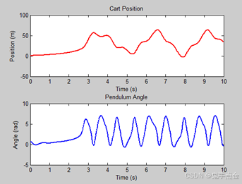
5. 仿真结果

运行仿真后，您将看到两个图形：

小车的位置：显示小车如何调整位置以帮助摆杆保持平衡。

摆杆的角度：显示摆杆如何调整角度并保持竖直。

6. 参数调节

为了更好地控制系统，您可能需要根据实际情况调整 PID 控制器的参数（Kp, Ki, Kd）。可以通过增大或减小这些参数来优化系统的响应速度、稳定性等。

7. 结论

该 MATLAB 仿真演示了如何使用串行 PID 控制器来控制倒立摆系统。通过调节 PID 参数，您可以实现更好的控制效果并使倒立摆系统稳定在竖直位置。