CNN简单实战：CIFAR10数据集物品分类（附完整代码）

前言

在上一篇CNN实战中（简单CNN网络实现手写数据集识别（附完整代码）），我们实现了mnist手写数据集识别，为了进一步巩固，本篇依然在公开数据集（CIFAR10）的基础上实现目标分类。下一篇将详细介绍如何自建分类数据集，并在自建的数据集上通过CNN实现分类。

由于上篇文章简单CNN网络实现手写数据集识别（附完整代码）已经详细介绍了模型参数的设置，因此这篇文章中不再做详细介绍，主要说明模型搭建流程。

CIFAR10数据集介绍

CIFAR10数据集共有60000个样本，每个样本都是一张32*32像素的RGB图像（彩色图像），每个RGB图像又必定分为3个通道（R通道、G通道、B通道）。这60000个样本被分成了50000个训练样本和10000个测试样本。
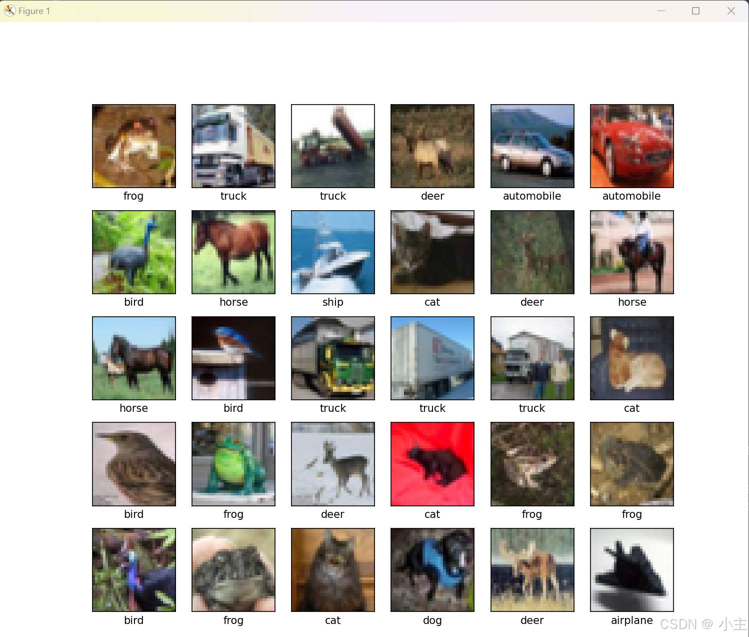
CIFAR10数据集是用来监督学习训练的，那么每个样本就一定都配备了一个标签值（用来区分这个样本是什么），不同类别的物体用不同的标签值，CIFAR10中有10类物体，标签值分别按照0~9来区分,他们分别是飞机（ airplane ）、汽车（ automobile ）、鸟（ bird ）、猫（ cat ）、鹿（ deer ）、狗（ dog ）、青蛙（ frog ）、马（ horse ）、船（ ship ）和卡车（ truck ）。

CIFAR-10 是一个广泛使用的图像数据集，它包含共 6 万张， 10 个类别的彩色图像，总共 6 万张图像。一下是该数据集的简单介绍：

1. 图像类别：数据集分为 10 个类别，每个类别包含 6000 张图像。类别包括：飞机、汽车、鸟、猫、鹿、狗、青蛙、马、船和卡车。

2. 数据分布：总共 6 万张图像，其中 5 万张用于训练，1 万张用于测试。每个类别在训练和测试集中是均匀分布的。

3. 图像规格：每张图像大小为 32x32 像素，彩色格式（即有 RGB 三个颜色通道）。

4. 文件格式：CIFAR-10 数据通常以 Python 格式提供，包含原始的图像数据和对应的标签，方便直接用于深度学习框架的加载和使用。

5. 数据来源：CIFAR-10 数据集由加拿大多伦多大学的 Alex Krizhevsky 和 Geoffrey Hinton 收集。它来源于 80 万张图像中的一部分，被整理成 10 个类别。

由于 CIFAR-10 的图像尺寸较小且数据量适中，它被广泛用于初学者的实验，以及模型在低分辨率图像上进行快速测试的基准。

CIFAR10数据集的内容，如图所示。

CNN实现CIFAR10数据集分类

接下来，一步一步对模型搭建过程进行介绍

1、导入相关模块

导入实验过程中会用到的模块

import tensorflow as tf
from tensorflow.keras import datasets, layers, models
import matplotlib.pyplot as plt

2、加载CIFAR10数据集

(train_images, train_labels), (test_images, test_labels) = datasets.cifar10.load_data()

3、数据预处理

这里主要是对数据进行归一化处理，将像素的值标准化至0到1的区间内。（为什么是除以255呢？由于图片的像素范围是0-255，我们把它变成0~1的范围，于是每张图像（训练集、测试集）都除以255。）

train_images, test_images = train_images / 255.0, test_images / 255.0

4、构建预测模型

模型中主要包含如下两个部分、
①特征提取：由卷积层与池化层实现
②实现分类：由全连接层实现，Dense 层等同于全连接层（此处，Dense 层的输入为向量（一维），但前面层的输出是3维的张量 (Tensor) 。因此需要将三维张量展开 (Flatten) 到1维，之后再传入一个或多个 Dense 层。）

model = models.Sequential([
    #特征提取：池化层与卷积层
    layers.Conv2D(32, (3, 3), activation='relu', input_shape=(32, 32, 3)), #32个3*3的卷积核
    layers.MaxPooling2D((2, 2)),
    layers.Conv2D(64, (3, 3), activation='relu'),
    layers.MaxPooling2D((2, 2)),
    layers.Conv2D(64, (3, 3), activation='relu'),

    #实现分类：全连接层
    layers.Flatten(),
    layers.Dense(64, activation='relu'),
    layers.Dense(10)
])

5、编译模型

编译模型主要是为模型指定损失函数loss、优化器 optimizer以及衡量指标metrics（通常用准确度accuracy 来衡量的）

model.compile(optimizer=tf.keras.optimizers.Adam(learning_rate=0.001),
              loss=tf.keras.losses.SparseCategoricalCrossentropy(from_logits=True),
              metrics=['accuracy'])

6、训练模型

使用fit对模型进行训练，并打印出模型效果。

#训练模型
history= model.fit(train_images, train_labels, epochs=30,
          validation_data=(test_images, test_labels))

plt.plot(history.history['accuracy'], label='accuracy')
plt.plot(history.history['val_accuracy'], label = 'val_accuracy')
plt.xlabel('Epoch')
plt.ylabel('Accuracy')
plt.ylim([0.5, 1])
plt.legend(loc='lower right')
plt.show()

test_loss, test_acc = model.evaluate(test_images,  test_labels, verbose=2)
print("测试集的准确度", test_acc)

模型效果如下（由于并没有详细调整模型参数，因此效果可能不太理想，对模型参数稍作修改可提高性能）：

通过模型进行预测

首先导入自己要预测的照片

# 载入我自己写的图片
img = Image.open(r'C:\Users\MCX2\Desktop\my_image.jpg')
plt.imshow(img)
plt.axis('off') # 不显示坐标
plt.show()

照片如下：

对照片大小进行预处理

# 把图片大小变成32×32,与CIFAR10数据集的图片大小相对应
image = np.array(img.resize((32, 32)))
plt.imshow(image)
plt.axis('off')
plt.show()

对处理后的照片进行预测

image = image.reshape((1, 32, 32, 3))
model = load_model('cifar10_model.h5')
prediction = model.predict(image)
print(prediction)

prediction_class = np.argmax(model.predict(image), axis=-1)
print('最终预测类别为：', prediction_class)

预测结果如下：

预测类别为[3]，这里我们可以看一下CIFAR10数据集的具体标签：class_names = [‘airplane’, ‘automobile’, ‘bird’, ‘cat’, ‘deer’, ‘dog’, ‘frog’, ‘horse’, ‘ship’, ‘truck’]，下标为3的标签为cat，预测正确。

训练部分完整代码

import tensorflow as tf
from tensorflow.keras import datasets, layers, models
import matplotlib.pyplot as plt

# 导入 CIFAR10 数据集
(train_images, train_labels), (test_images, test_labels) = datasets.cifar10.load_data()


class_names = ['airplane', 'automobile', 'bird', 'cat', 'deer',
               'dog', 'frog', 'horse', 'ship', 'truck']

plt.figure(figsize=(10,10))
for i in range(30):
    plt.subplot(5,6,i+1)
    plt.xticks([])
    plt.yticks([])
    plt.grid(False)
    plt.imshow(train_images[i], cmap=plt.cm.binary)
    # 由于 CIFAR 的标签是 array， 因此需要额外的索引（index）。
    plt.xlabel(class_names[train_labels[i][0]])
plt.show()

train_images, test_images = train_images / 255.0, test_images / 255.0 #数据归一化处理

#构建模型
model = models.Sequential([
    #特征提取：池化层与卷积层
    layers.Conv2D(32, (3, 3), activation='relu', input_shape=(32, 32, 3)), #32个3*3的卷积核
    layers.MaxPooling2D((2, 2)),
    layers.Conv2D(64, (3, 3), activation='relu'),
    layers.MaxPooling2D((2, 2)),
    layers.Conv2D(64, (3, 3), activation='relu'),

    #实现分类：全连接层
    layers.Flatten(),
    layers.Dense(64, activation='relu'),
    layers.Dense(10)
])

#编译模型
model.compile(optimizer=tf.keras.optimizers.Adam(learning_rate=0.001),
              loss=tf.keras.losses.SparseCategoricalCrossentropy(from_logits=True),
              metrics=['accuracy'])

#训练模型
history= model.fit(train_images, train_labels, epochs=10,
          validation_data=(test_images, test_labels))

#test_loss, test_acc = model.evaluate(test_images,  test_labels, verbose=2) #评估模型在测试集上的性能

plt.plot(history.history['accuracy'], label='accuracy')
plt.plot(history.history['val_accuracy'], label = 'val_accuracy')
plt.xlabel('Epoch')
plt.ylabel('Accuracy')
plt.ylim([0.5, 1])
plt.legend(loc='lower right')
plt.show()

test_loss, test_acc = model.evaluate(test_images,  test_labels, verbose=2)
print("测试集的准确度", test_acc)

model.save("cifar10_model.h5")

预测部分完整代码

import tensorflow as tf
from tensorflow.keras.models import load_model
import matplotlib.pyplot as plt
from PIL import Image
import numpy as np



# 载入我自己写的图片
img = Image.open(r'C:\Users\MCX2\Desktop\my_image.jpg')
plt.imshow(img)
plt.axis('off') # 不显示坐标
plt.show()

# 把图片大小变成32×32,与CIFAR10数据集的图片大小相对应
image = np.array(img.resize((32, 32)))
plt.imshow(image)
plt.axis('off')
plt.show()


image = image.reshape((1, 32, 32, 3))
model = load_model('cifar10_model.h5')
prediction = model.predict(image)
print(prediction)

prediction_class = np.argmax(model.predict(image), axis=-1)
print('最终预测类别为：', prediction_class)