


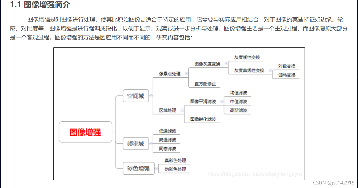
 本文详细介绍了一系列图像处理技术的应用,包括图像的加载与展示、旋转、缩放、水平及上下反转等基本操作,进一步探讨了灰度化、二值化、直方图均衡化等图像增强方法,并介绍了均值滤波与高斯滤波两种常见的图像平滑技术。
1.打开图像
import os
import matplotlib.image as mpimg
import numpy as np
import matplotlib.pyplot as plt #显示照片
from PIL import Image

cwd = os.getcwd()   # 获得当前工作路径
print(cwd)
path = cwd + "/images"
valid_exts = [".jpg", ".gif", ".png", ".tga", ".jpeg"]

print('%d files in %s'%(len(os.listdir(path)), path))

imgs =[]
names =[]
for f in os.listdir(path):
    ext = os.path.splitext(f)[1]   #ext:('1', '.jpg')  ext[1]:  .jpg
    if ext.lower() not in valid_exts :
        continue
    fullpath = os.path.join(path, f)
    imgs.append(mpimg.imread(fullpath))
    names.append(os.path.splitext(f)[0]+os.path.splitext(f)[1])


print('%d images loaded'%(len(imgs)))

nimgs = len (imgs)
randidx = np.sort(np.random.randint(nimgs, size=3))
print(randidx)

print('Type of imgs :', type(imgs))
print('Length of imgs :', len(imgs))

for curr_img, curr_name, i in zip([imgs[j] for j in randidx], [names[j] for j in randidx], range(len(randidx))):
    print('[%d] Type of curr_img: %s'%(i, type(curr_img)))
    print('Name is :%s'%(curr_name))
    print('size of curr_img: %s '%(curr_img.shape,)) # ,逗号
import matplotlib.image as mpimg
mpimg.imread()
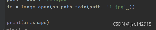
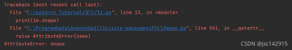
可以用 im.shape
from PIL import Image
利用Image
valid_exts1=["jpg", "gif", "png", "tga", "jpeg"]
ims = input('请输入文件名:')
print(ims.split('.', 1)[1])
while ims.split('.', 1)[1] in valid_exts1:
    im = mpimg.imread(os.path.join(path, ims ))
    plt.imshow(im)
    print(im.shape)
    plt.show()
    break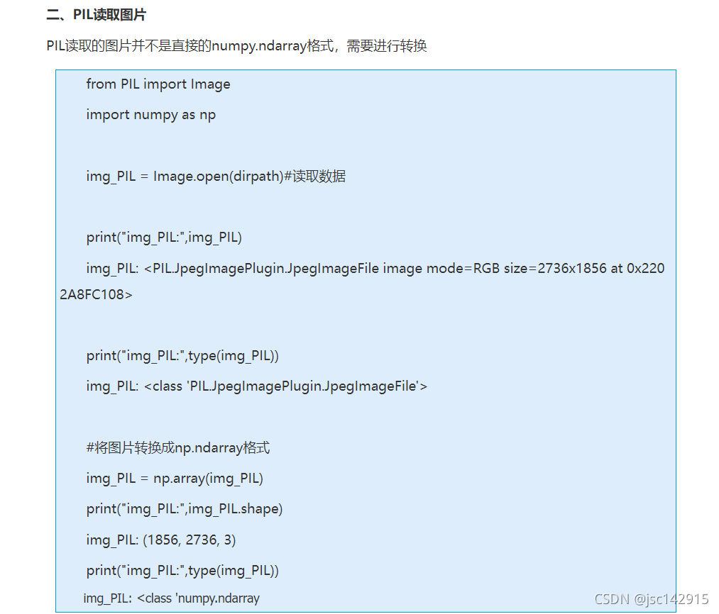
2. 旋转(PIL)
#旋转
im = Image.open(os.path.join(path, ims ))
angle = int(input('请输入旋转角度:'))
im_rotate = im.rotate(angle=angle)
im_rotate.show()
plt.imshow(im_rotate)
plt.show()
3.缩放
p = float(input('请输入缩放比例(0-1):'))
(x, y) = im.size
x_s = x *p
y_s = y *p
out = im.resize((x_s, y_s), Image.ANTIALIAS)
out.show()
#im_resize = im.resize((128, 128)) 直接输入所需的大小
补充:os.walk()用类似于深度遍历的方式遍历文件夹中的子文件夹以及文件。最基本的显示方式为(root_path,[file_dirs],[files]),以元组为单位区分每一层的,每一层又分成三个部分根目录路径、本目录中文件夹名字、本目录中文件名字。
for root, dirs, files in os.walk(image_path):
print("root:"+root)
print(dirs)
print(files)
4.水平反转
out1 = im.transpose(Image.FLIP_LEFT_RIGHT)  # 实现翻转
out1.show()
 5.上下反转
out2 = im.transpose(Image.FLIP_TOP_BOTTOM)  #上下反转

out2.show() 
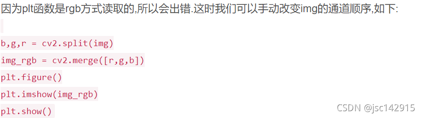
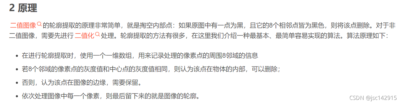
6.提取轮廓
cv2.imread()-----opencv读取图像为b,g,r方法
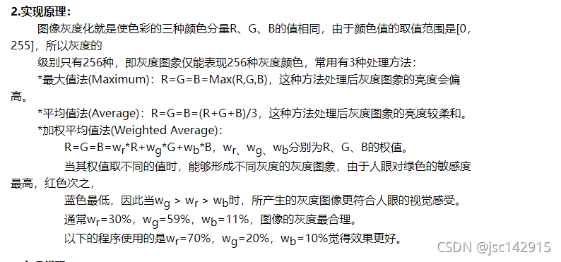
灰度化与二值化的区别
灰度化:在RGB模型中,如果R=G=B时,则彩色表示一种灰度颜色,其中R=G=B的值叫灰度值,因此,灰度图像每个像素只需一个字节存放灰度值(又称强度值、亮度值),灰度范围为0-255。一般常用的是加权平均法来获取每个像素点的灰度值。
二值化:图像的二值化,就是将图像上的像素点的灰度值设置为0或255,也就是将整个图像呈现出明显的只有黑和白的视觉效果
img = cv2.imread(r'F:\pytorch Tutorial\study\images\1.jpg')
cv2.imshow('Example',img)
cv2.waitKey(0)

gray_img = cv2.cvtColor(img,cv2.COLOR_BGR2GRAY) #灰度化
cv2.imshow('Example1',gray_img)
cv2.waitKey(0)

#二值化
def get_binary_img(img):
    # gray img to bin image
    bin_img = np.zeros(shape=(img.shape), dtype=np.uint8)
    h = img.shape[0]
    w = img.shape[1]
    for i in range(h):
        for j in range(w):
            bin_img[i][j] = 255 if img[i][j] > 127 else 0
    return bin_img
# 调用
bin_img = get_binary_img(gray_img)

cv2.imshow('Example2',bin_img )
cv2.waitKey(0)


def get_contour(bin_img):
    # get contour
    contour_img = np.zeros(shape=(bin_img.shape),dtype=np.uint8)
    contour_img += 255
    h = bin_img.shape[0]
    w = bin_img.shape[1]
    for i in range(1,h-1):
        for j in range(1,w-1):
            if(bin_img[i][j]==0):
                contour_img[i][j] = 0
                sum = 0
                sum += bin_img[i - 1][j + 1] #判断此像素点附近八个点的值是否为0
                sum += bin_img[i][j + 1]
                sum += bin_img[i + 1][j + 1]
                sum += bin_img[i - 1][j]
                sum += bin_img[i + 1][j]
                sum += bin_img[i - 1][j - 1]
                sum += bin_img[i][j - 1]
                sum += bin_img[i + 1][j - 1]
                if sum ==  0:
                    contour_img[i][j] = 255

    return contour_img
# 调用
contour_img = get_contour(bin_img)

cv2.imshow('Example3',contour_img)
cv2.waitKey(0)
7.灰度图反相处理
#反相处理
#(x_1,y_1)=gray_img.size

img = cv2.imread(r'F:\pytorch Tutorial\study\images\1.jpg')
cv2.imshow('Example',img)
cv2.waitKey(0)

gray_img = cv2.cvtColor(img,cv2.COLOR_BGR2GRAY) #灰度化
cv2.imshow('Example1',gray_img)
cv2.waitKey(0)
a=np.ones_like(gray_img, dtype=np.int32) *255
b = a- gray_img
plt.imshow(b,cmap='gray')
plt.show()
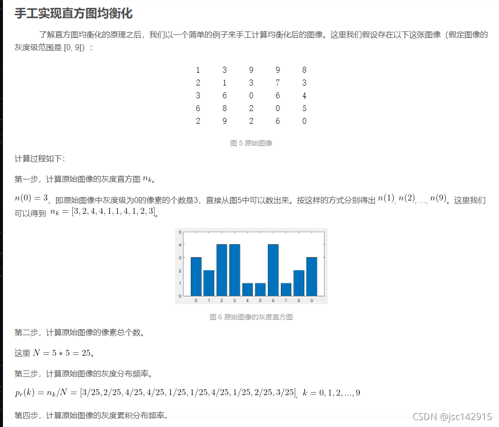
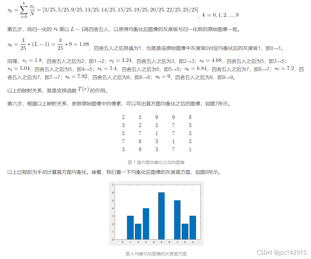
8.python直方图均衡化

直方图均衡化就是把一已知灰度概率分布的图像经过一种变换使之演变成一幅具有均匀灰度概率分布的新图像
灰度处理
问题1:如何计算直方图?
对于8位灰度图来说,颜色有256级,统计每级的个数,然后把结果用图表表示出来就可以了
import cv2
import matplotlib.pyplot as plt
import numpy as np
import os
gray_level = 256
def piexl_im(img):
assert isinstance(img, np.ndarray)
(height, width) = img.shape
prob = np.zeros(shape=(256))
for i in range(height):
for j in range(width):
k = img[i,j] # 一点的像素值
prob[k] = prob[k]+1
return prob
def piexl_prob(img):
assert isinstance(img, np.ndarray)
(height, width) = img.shape
prob = np.zeros(shape=(256))
for i in range(height):
for j in range(width):
k = img[i,j] # 一点的像素值
prob[k] = prob[k]+1
prob= prob/(height * width)
return prob
img = cv2.imread('1.jpg')
gray_img = cv2.cvtColor(img,cv2.COLOR_BGR2GRAY) #灰度化
x=piexl_im(gray_img)
a= range(256)
plt.bar(a, x,width=0.2)
plt.show()
probably = piexl_prob(gray_img)
def probability_to_histogram(img, prob):
prob = np.cumsum(prob) # 累计概率
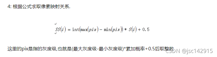
img_map = [int(255 * prob[i] + 0.5) for i in range(256)] # 像素值映射
# 像素值替换
assert isinstance(img, np.ndarray)
r, c = img.shape
for ri in range(r):
for ci in range(c):
img[ri, ci] = img_map[img[ri, ci]]
return img
def plot(y, name):
"""
画直方图,len(y)==gray_level
:param y: 概率值
:param name:
:return:
"""
plt.figure(num=name)
plt.bar([i for i in range(gray_level)], y, width=1)
img = cv2.imread("1.jpg", 0) # 读取灰度图
prob = piexl_prob(img)
plot(prob, "原图直方图")
# 直方图均衡化
img = probability_to_histogram(img, prob)
cv2.imwrite("source_hist.jpg", img) # 保存图像
prob = piexl_prob(img)
plot(prob, "直方图均衡化结果")
plt.show()
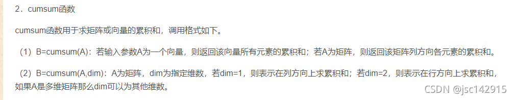
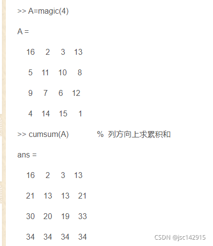
补充: cumsum()
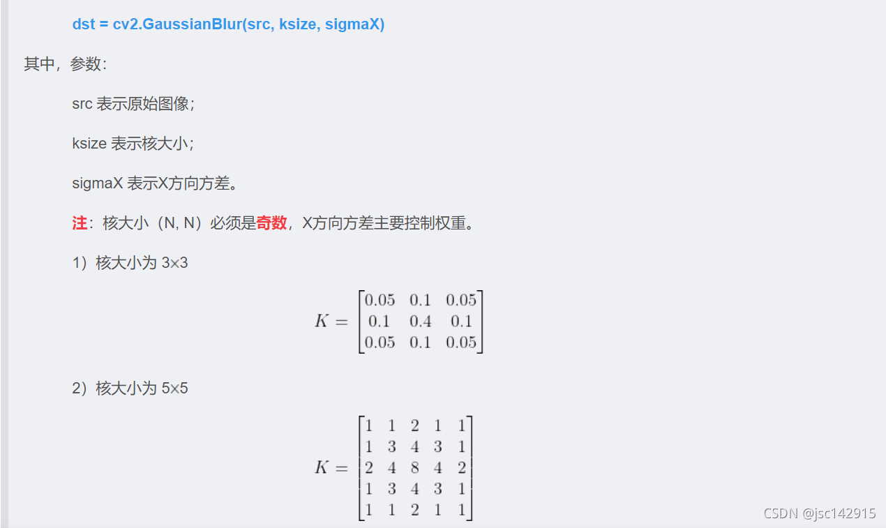
9.均值滤波、高斯滤波
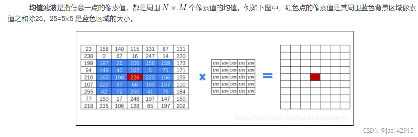
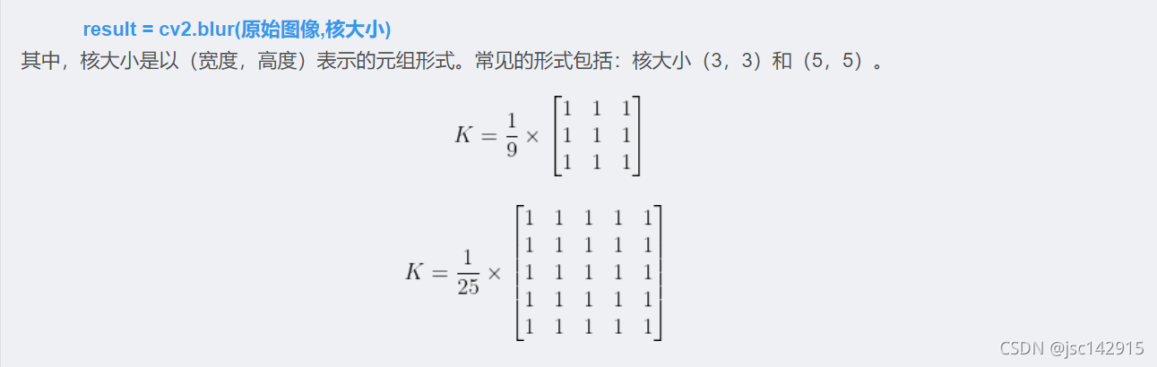
cv.blur( 图像, (核3,3))------》改变核的大小可以改变滤波强度
高斯滤波
#自定义均值滤波

def mean_blur(img,kernel_size=3):
    h, w, c = img.shape

    #零填充
    k = kernel_size//2
    a = np.zeros((h + 2*k,w + 2*k,c),dtype=np.float)
    a[k:k + h, k:k + w] = img.copy().astype(np.float)

    #卷积
    temp= a.copy()
    for y in range(h):
        for x in range(w):
            for ci in range(c):
                a[k+y,k+x,ci]=np.mean(temp[y:y+kernel_size,x:x+kernel_size,ci])

    out = a[k:k + h, k:k + w].astype(np.uint8)
    return out
#自定义高斯滤波
def gaussian_filter(img, K_size=3, sigma=1.3):
if len(img.shape) == 3:
H, W, C = img.shape
else:
img = np.expand_dims(img, axis=-1)
H, W, C = img.shape
## Zero padding
pad = K_size // 2
out = np.zeros((H + pad * 2, W + pad * 2, C), dtype=np.float)
out[pad: pad + H, pad: pad + W] = img.copy().astype(np.float)
## prepare Kernel
K = np.zeros((K_size, K_size), dtype=np.float)
for x in range(-pad, -pad + K_size):
for y in range(-pad, -pad + K_size):
K[y + pad, x + pad] = np.exp(-(x ** 2 + y ** 2) / (2 * (sigma ** 2)))
K /= (2 * np.pi * sigma * sigma)
K /= K.sum()
tmp = out.copy()
# filtering
for y in range(H):
for x in range(W):
for c in range(C):
out[pad + y, pad + x, c] = np.sum(K * tmp[y: y + K_size, x: x + K_size, c])
out = np.clip(out, 0, 255)
out = out[pad: pad + H, pad: pad + W].astype(np.uint8)
return out
参考文献:
实例说明图像的灰度化和二值化的区别 - 云+社区 - 腾讯云
【深度好文】Python图像处理之目标物体轮廓提取_sgzqc的专栏-优快云博客 Opencv-python(cv2)图像读取、显示与保存,看这一篇就够了_风雪夜归人o的博客-优快云博客
数字图像处理(11): 图像平滑 (均值滤波、中值滤波和高斯滤波)_TechArtisan6的博客-优快云博客
手动实现均值滤波(python)_陨星落云的博客-优快云博客_均值滤波python
高斯滤波详解 python实现高斯滤波_Ibelievesunshine的博客-优快云博客


 3638
3638

 被折叠的 条评论
为什么被折叠?
被折叠的 条评论
为什么被折叠?
 到【灌水乐园】发言


