


第一步:下载ERA5日数据并进行裁剪
在GIS中完成,注意所有的图片具有相同的分辨率和投影,以及格子数量也需要一样
第二步:将其进行tif到nc格式的转变,具体代码如下:
import rasterio
import numpy as np
import os
from netCDF4 import Dataset
import datetime

def is_leap_year(year):
    return (year % 4 == 0 and year % 100 != 0) or (year % 400 == 0)

tif_folder = r'F:\CMIP6\MRSOS_clipped_2'
years = range(1981, 2021)

all_data = []
time_values = []  # 存储数值型时间
base_date = datetime.date(2015, 1, 1)

# 获取地理信息并提前保存CRS
with rasterio.open(os.path.join(tif_folder, f"SM2_5000_{years[0]}.tif")) as src:
    profile = src.profile
    rows, cols = src.shape
    transform = src.transform  # Affine(a, b, c, d, e, f)
    crs_wkt = src.crs.to_wkt()
    nodata = profile['nodata']

# ✅ 正确生成经纬度坐标
lat_values = [transform.f + i * transform.e for i in range(rows)]  # 纬度从左上角开始递减
lon_values = [transform.c + j * transform.a for j in range(cols)]  # 经度从左上角开始递增

# 读取数据并生成时间序列
for year in years:
    tif_file = os.path.join(tif_folder, f"SM2_5000_{year}.tif")
    with rasterio.open(tif_file) as src:
        data = src.read()
        days_in_year = 366 if is_leap_year(year) else 365

        if data.shape[0] != days_in_year:
            raise ValueError(f"文件 {year}.tif 波段数不符")

        all_data.extend([data[i] for i in range(days_in_year)])

        # 生成当前年的时间序列
        start_date = datetime.date(year, 1, 1)
        for day in range(days_in_year):
            current_date = start_date + datetime.timedelta(days=day)
            delta = (current_date - base_date).days
            time_values.append(delta)

# 转换为numpy数组
all_data = np.array(all_data)

# 创建NetCDF文件
nc_file = r'F:\CMIP6\mrsos_daily_data_2015_2020.nc'
with Dataset(nc_file, 'w', format='NETCDF4') as nc:
    # 定义维度
    nc.createDimension('time', len(time_values))
    nc.createDimension('lat', rows)
    nc.createDimension('lon', cols)

    # 时间变量
    time_var = nc.createVariable('time', 'i4', ('time',))
    time_var.units = "days since 2015-01-01"
    time_var.calendar = "gregorian"
    time_var[:] = time_values

    # 经纬度变量
    lat_var = nc.createVariable('lat', 'f4', ('lat',))
    lon_var = nc.createVariable('lon', 'f4', ('lon',))
    lat_var[:] = lat_values
    lon_var[:] = lon_values
    lat_var.units = "degrees_north"
    lon_var.units = "degrees_east"

    # 坐标系变量
    crs_var = nc.createVariable('crs', 'i4')
    crs_var.spatial_ref = crs_wkt
    crs_var.GeoTransform = " ".join(map(str, transform.to_gdal()))

    # 数据变量
    data_var = nc.createVariable('sm', 'f4', ('time', 'lat', 'lon'),
                                fill_value=nodata)
    data_var.units = "kg/m²"
    data_var.long_name = "Soil Moisture"
    data_var.grid_mapping = "crs"
    data_var[:] = all_data

print(f"成功创建: {nc_file}")
第三步,进行不同模式历史数据的重采样:我的数据是1981-2014年这个阶段,所以全部进行这个阶段的重采样:
import xarray as xr
import os
import glob

# 载入源文件和目标文件
source_file = r'F:\CMIP6_1\TAS\historical\tas_day_BCC-CSM2-MR_historical_r1i1p1f1_gn_19810101-20141231.nc'
target_file = r'I:\CMIP6_4\ERA5_daily_tas_1981-2014_12410.nc'

# 打开数据文件
source_ds = xr.open_dataset(source_file)
target_ds = xr.open_dataset(target_file)

# 获取目标文件的网格分辨率
target_lat = target_ds['lat']  # 假设纬度变量名为lat
target_lon = target_ds['lon']  # 假设经度变量名为lon

# 假设源数据的时间维度为'time',并且每一层数据需要重采样
source_data = source_ds['tas']  # 假设目标变量名为'mrsos',你可以根据实际情况修改

# 创建一个新的空的数组来存储重采样的数据
resampled_data = []

# 遍历时间维度中的每一层数据,并进行重采样
for t in range(len(source_data.time)):
    # 获取当前时间步的数据
    layer = source_data.isel(time=t)

    # 对该层数据进行重采样
    resampled_layer = layer.interp(lat=target_lat, lon=target_lon)

    # 将重采样的层添加到列表中
    resampled_data.append(resampled_layer)

# 将所有重采样后的数据堆叠在一起,重新构建一个数据集
resampled_data = xr.concat(resampled_data, dim='time')

# 保存重采样后的数据
output_file = r'F:\CMIP6_1\TAS\historical\resample_tas_day_BCC-CSM2-MR_historical_r1i1p1f1_gn_19810101-20141231.nc'
resampled_data.to_netcdf(output_file)

print(f"重采样后的数据已保存至 {output_file}")
第四步,进行随机森林模拟进行历史数据降尺度,机器学习,为预测做准备:
import numpy as np
import xarray as xr
from sklearn.ensemble import RandomForestRegressor
from sklearn.model_selection import train_test_split
from sklearn.metrics import mean_squared_error
from joblib import dump

# ========== 1. 读取数据 ==========
canesm5 = xr.open_dataset(r"F:\CMIP6_1\TAS\historical\resample_tas_day_CanESM5_historical_r1i1p1f1_gn_19810101-20141231.nc", decode_times=False)["tas"]
era5 = xr.open_dataset("I:/CMIP6_4/ERA5_daily_tas_1981-2014_12410.nc", decode_times=False)["tas"]

# ========== 2. 直接按索引对齐时间维度 ==========
min_len = min(canesm5.sizes['time'], era5.sizes['time'])
canesm5 = canesm5.isel(time=slice(0, min_len))
era5 = era5.isel(time=slice(0, min_len))

print(f"✅ 直接按索引对齐,共使用时间步数:{min_len}")

# ========== 3. 标准化 ==========
canesm5_mean = canesm5.mean().item()
canesm5_std = canesm5.std().item()
era5_mean = era5.mean().item()
era5_std = era5.std().item()

canesm5_norm = (canesm5 - canesm5_mean) / canesm5_std
era5_norm = (era5 - era5_mean) / era5_std

# ========== 4. 展平并清洗 NaN ==========
X = canesm5_norm.values.reshape(-1)
y = era5_norm.values.reshape(-1)
mask = ~np.isnan(X) & ~np.isnan(y)
X_valid = X[mask]
y_valid = y[mask]

print(f"🎯 有效训练样本数: {len(X_valid)}")

# ========== 5. 限制样本数 ==========
if len(X_valid) > 2_000_000:
    idx = np.random.choice(len(X_valid), size=2_000_000, replace=False)
    X_valid = X_valid[idx]
    y_valid = y_valid[idx]

# ========== 6. 拆分训练集 / 测试集 ==========
X_train, X_test, y_train, y_test = train_test_split(
    X_valid, y_valid, test_size=0.2, random_state=42
)

# ========== 7. 模型训练 ==========
model = RandomForestRegressor(n_estimators=40, max_depth=12, n_jobs=-1, random_state=42)
model.fit(X_train.reshape(-1, 1), y_train)

# ========== 8. 评估 ==========
y_pred = model.predict(X_test.reshape(-1, 1))
rmse = np.sqrt(mean_squared_error(y_test, y_pred))
print(f"✅ 模型训练完成!RMSE: {rmse:.4f}")

# ========== 9. 保存模型和参数 ==========
dump(model, r"F:\CMIP6_1\TAS\RF\downscale_RF_model_CanESM_final.joblib")
np.savez(r"F:\CMIP6_1\TAS\RF\standardization_params_CanESM_final.npz",
         mean_input=canesm5_mean,
         std_input=canesm5_std,
         mean_target=era5_mean,
         std_target=era5_std)
print("✅ 模型和参数保存完毕")
第五步,开始对未来进行降尺度:
import numpy as np
import xarray as xr
from joblib import load
from tqdm import tqdm  # 进度条支持

# ========== 1. 加载预训练模型和参数 ==========
model = load(r"F:\CMIP6_1\TAS\RF\downscale_RF_model_CanESM_final.joblib")
params = np.load(r"F:\CMIP6_1\TAS\RF\standardization_params_CanESM_final.npz")

# 提取标准化参数
canesm5_mean = params['mean_input']
canesm5_std = params['std_input']
era5_mean = params['mean_target']
era5_std = params['std_target']

# ========== 2. 读取未来气候数据 ==========
file_path=r"D:\CMIP6_3\TEM\resample_xinjiang_tas_day_CanESM5_ssp245_r1i1p1f1_gn_20150101-20481231_cropped.nc"
future_ds = xr.open_dataset(file_path,
                           decode_times=False)["tas"]

# ========== 3. 数据预处理 ==========
# 标准化处理(使用历史数据的参数)
future_norm = (future_ds - canesm5_mean) / canesm5_std

# 初始化存储矩阵
predicted_data = np.full(future_ds.shape, np.nan)

# ========== 4. 逐时间步预测 ==========
for i in tqdm(range(future_ds.shape[0]), desc='降尺度处理'):
    # 获取当前时间步数据
    time_slice = future_norm[i].values.reshape(-1)

    # 创建有效数据掩膜
    valid_mask = ~np.isnan(time_slice)
    X_valid = time_slice[valid_mask]

    # 跳过全NaN的时间步
    if len(X_valid) == 0:
        continue

    # 执行预测
    y_pred = model.predict(X_valid.reshape(-1, 1))

    # 逆标准化
    y_restored = y_pred * era5_std + era5_mean

    # 重构空间矩阵
    reconstructed = np.full_like(time_slice, np.nan)
    reconstructed[valid_mask] = y_restored
    predicted_data[i] = reconstructed.reshape(future_ds.shape[1:])

# ========== 5. 构建输出数据集 ==========
# 创建时间坐标(假设原始时间单位为日,需确认)
start_year = int(file_path[68:72])
print(start_year)
end_year = int(file_path[77:81])
print(end_year)
time_coords = xr.cftime_range(start=f"{start_year}-01-01",
                             end=f"{end_year}-12-31",
                             freq="D")

# 创建DataArray
output_da = xr.DataArray(
    data=predicted_data,
    dims=('time', 'lat', 'lon'),
    coords={
        'time': time_coords[:future_ds.shape[0]],  # 确保长度匹配
        'lat': future_ds.lat.values,
        'lon': future_ds.lon.values
    },
    attrs={
        'long_name': 'downscaled_temperature',
        'units': '℃/day',
        'method': 'RandomForest downscaling'
    }
)

# ========== 6. 保存结果 ==========
output_ds = xr.Dataset({'mrsos': output_da})
output_ds.to_netcdf(r"D:\CMIP6_3\TEM\final\CanESM5\downscaling_xinjiang_tas_day_CanESM5_ssp245_r1i1p1f1_gn_20150101-20481231.nc")
print("✅ 降尺度完成!结果已保存至指定路径")
第六步,降尺度后的数据结果检查
import xarray as xr

# 加载所有情景数据
ssp126 = xr.open_dataset(r'H:\CMIP6_2\down_scaling\MIROC6\future\downscaling_xinjiang_mrsos_day_MIROC6_ssp126_r1i1p1f1_gn_20150101-20481231.nc')
ssp245 = xr.open_dataset(r'H:\CMIP6_2\down_scaling\MIROC6\future\downscaling_xinjiang_mrsos_day_MIROC6_ssp245_r1i1p1f1_gn_20150101-20481231.nc')
ssp370 = xr.open_dataset(r'H:\CMIP6_2\down_scaling\MIROC6\future\downscaling_xinjiang_mrsos_day_MIROC6_ssp370_r1i1p1f1_gn_20150101-20481231.nc')
ssp585 = xr.open_dataset(r'H:\CMIP6_2\down_scaling\MIROC6\future\downscaling_xinjiang_mrsos_day_MIROC6_ssp585_r1i1p1f1_gn_20150101-20481231.nc')

# 示例:计算每个时间层的全局空间均值(假设变量名为 'mrsos')
mean_126 = ssp126['mrsos'].mean(dim=['lat', 'lon'])  # 空间平均
mean_245 = ssp245['mrsos'].mean(dim=['lat', 'lon'])
mean_370 = ssp370['mrsos'].mean(dim=['lat', 'lon'])
mean_585 = ssp585['mrsos'].mean(dim=['lat', 'lon'])

import matplotlib.pyplot as plt

plt.figure(figsize=(12, 6))
mean_126.plot(label='SSP126', color='blue')
mean_245.plot(label='SSP245', color='green')
mean_370.plot(label='SSP370', color='orange')
mean_585.plot(label='SSP585', color='red')
plt.title('Comparison of Soil Moisture (mrsos) Across SSP Scenarios')
plt.ylabel('Mean Value')
plt.legend()
plt.show()
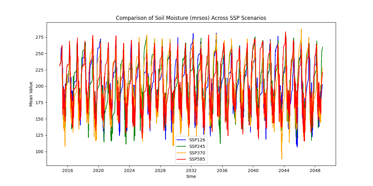
到此为止,降尺度结束~


 1万+
1万+

 被折叠的 条评论
为什么被折叠?
被折叠的 条评论
为什么被折叠?
 到【灌水乐园】发言


