Batch Gradient Descent

Batch Gradient Descent

We use linear regression as example to explain this optimization algorithm.

1. Formula

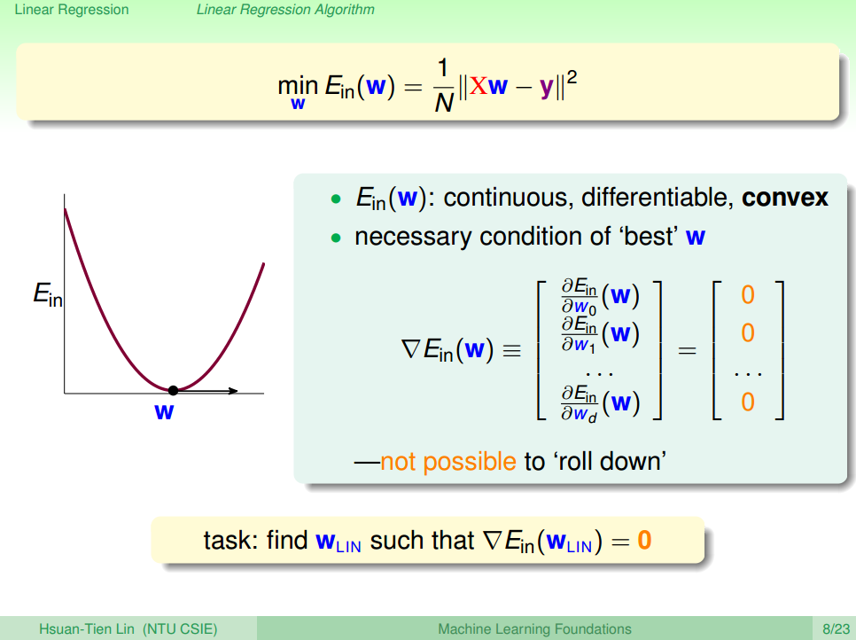
1.1. Cost Function

We prefer residual sum of squared to evaluate linear regression.

$$\begin{align} J(\theta) &= \frac{1}{2m} \sum\limits_{i=1}^{n} \left[ h_{\theta}(x_i) - y_i \right] ^ 2 \end{align}$$

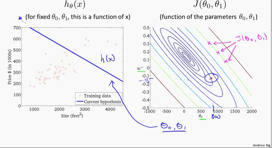
1.2. Visualize Cost Function

E.g. 1 :

one parameter only $\theta_1$ –> $h_{\theta}(x) = \theta_1 x_1$

1. Learning Curve 1 ^[1]

E.g. 2 :

two parameters $\theta_0, \theta_1$ –> $h_{\theta}(x) = \theta_0 + \theta_1 x_1$

2. Learning Curve 2 ^[2]

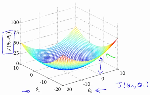
Switch to contour plot

3. Learning Curve 2 - contour^[2]

1.3. Gradient Descent Formula

For all $\theta_i$

$$\begin{align} \frac{\partial J_\theta}{\partial \theta_i} = \frac{1}{m} \sum\limits_{i=1}^{n} \left[ h_{\theta}(x_i) - y_i \right] \cdot (x_i) \end{align}$$

E.g.,
two parameters $\theta_0, \theta_1$ –> $h_{\theta}(x) = \theta_0 + \theta_1 x_1$

For i = 0 :

$$\frac{\partial J_\theta}{\partial \theta_0} = \frac{1}{m} \sum\limits_{i=1}^{n} \left[ h_{\theta}(x_i) - y_i \right] \cdot (x_0)$$

For i = 1:

$$\frac{\partial J_\theta}{\partial \theta_1} = \frac{1}{m} \sum\limits_{i=1}^{n} \left[ h_{\theta}(x_i) - y_i \right]\cdot (x_1)$$

% Octave
%% =================== Gradient Descent ===================
% Add a column(x0) of ones to X

X = [ones(len, 1), data(:,1)];
theta = zeros(2, 1);
alpha = 0.01;
ITERATION = 1500;
jTheta = zeros(ITERATION, 1);

for iter = 1:ITERATION
    % Perform a single gradient descent on the parameter vector
    % Note: since the theta will be updated, a tempTheta is needed to store the data.
    tempTheta = theta;
    theta(1) = theta(1) - (alpha / len) * (sum(X * tempTheta - Y));  % ignore the X(:,1) since the values are all ones.
    theta(2) = theta(2) - (alpha / len) * (sum((X * tempTheta - Y) .* X(:,2)));

    %% =================== Compute Cost ===================
    jTheta(iter) = sum((X * theta - Y) .^ 2) / (2 * len);
endfor

2. Algorithm

For all $\theta_i$

$$\begin{align} \theta_i := \theta_i - \alpha \frac{\partial}{\partial \theta_i} J(\theta_1, \theta_2, \dots ,\theta_n) \end{align}$$

E.g.,
two parameters $\theta_0, \theta_1$ –> $h_{\theta}(x) = \theta_0 + \theta_1 x_1$

For i = 0 :

$$\begin{align} \theta_0 := \theta_0 - \alpha \frac{1}{m} \sum\limits_{i=1}^{n} \left[ h_{\theta}(x_i) - y_i \right] \end{align}$$

For i = 1 :

$$\begin{align} \theta_1 := \theta_1 - \alpha \frac{1}{m} \sum\limits_{i=1}^{n} \left[ h_{\theta}(x_i) - y_i \right] \cdot (x_1) \end{align}$$

Iterative for multiple times (depends on data content, data size and step size). Finally, we could see the result as below.

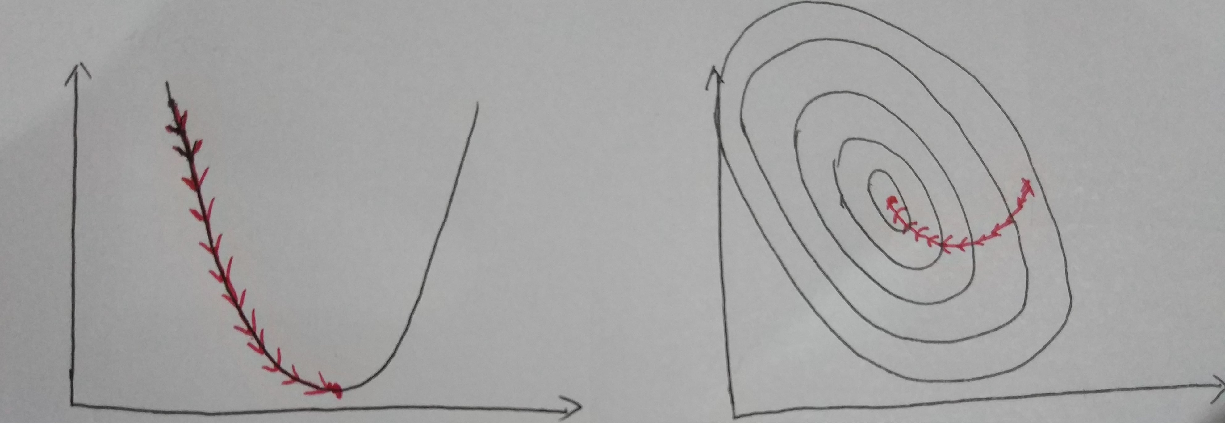
Visualize Convergence

3. Analyze

Pros	Cons
Controllable by manuplate stepsize, datasize	Computing effort is large
Easy to program

4. How to Choose Step Size?

Choose an approriate step size is significant. If the step size is too small, it doesn’t hurt the result, but it took even more times to converge. If the step size is too large, it may cause the algorithm diverge (not converge).

The graph below shows that the value is not converge since the step size is too big.

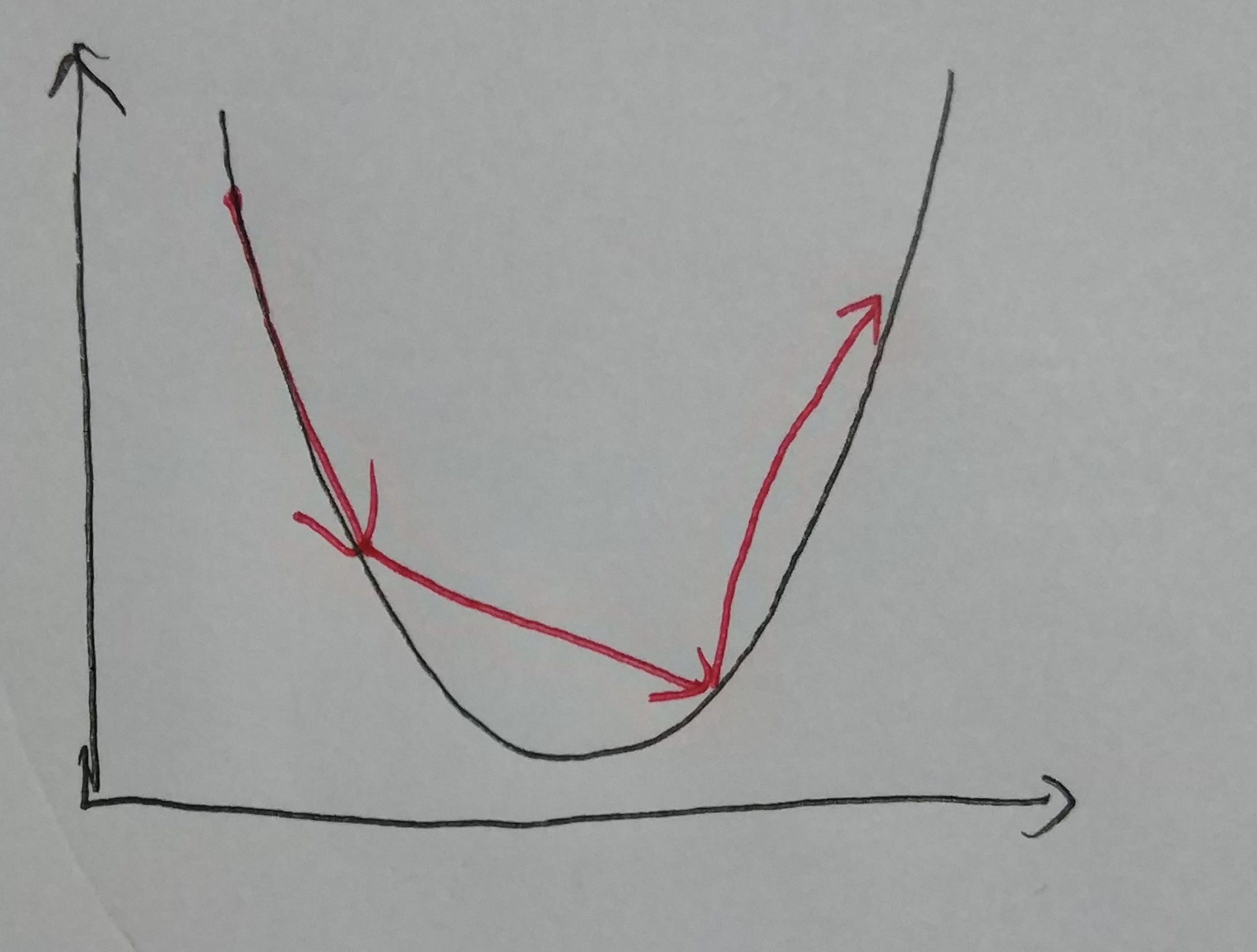
Large Step Size

The best way, as far as I know, is to decrease the step size according to the iteration times.

E.g.,

$\alpha^{(t+1)} = \frac{\alpha^{t}}{t}$

or

$\alpha^{(t+1)} = \frac{\alpha^{t}}{\sqrt t}$

Reference

1. 机器学习基石(台湾大学-林轩田)\lecture_slides-09_handout.pdf

2. Coursera-Standard Ford CS229: Machine Learning - Andrew Ng