


 本博客介绍了一个基于CIFAR-10数据集的图像分类模型的构建过程,包括数据预处理、增强、模型搭建、训练及评估。模型采用深度卷积神经网络,利用批量归一化和残差连接提升性能。
import matplotlib.pyplot as plt
from sklearn.datasets import load_iris
from sklearn.decomposition import PCA
from sklearn.model_selection import train_test_split
from sklearn.preprocessing import StandardScaler
import tensorflow as tf
import numpy as np
import pandas as pd
import os
import glob
import pickle
import scipy.misc
#from tqdm import tqdm
num_classes = 10
(X_train, y_train), (X_test, y_test) = tf.keras.datasets.cifar10.load_data()
X_train.shape,y_train.shape,X_test.shape,y_test.shape
((50000, 32, 32, 3), (50000, 1), (10000, 32, 32, 3), (10000, 1))
y_train = tf.keras.utils.to_categorical(y_train, num_classes)
y_test = tf.keras.utils.to_categorical(y_test, num_classes)
#第二步骤:构造ImageDataGenerator类的对象,通过参数指定要进行处理项目
#对数据进行预处理,注意这里不是一次性要将所有的数据进行处理完,而是在后面的代码中进行逐批次处理
datagen = tf.keras.preprocessing.image.ImageDataGenerator(
    rescale=1./255,
    featurewise_center=True,
    featurewise_std_normalization=True,
    rotation_range=40, # 角度值,0~180,图像旋转
    width_shift_range=0.2, # 水平平移,相对总宽度的比例
    height_shift_range=0.2, # 垂直平移,相对总高度的比例
    shear_range=0.2, # 随机错切换角度
    zoom_range=0.2, # 随机缩放范围
    horizontal_flip=True, # 一半图像水平翻转
    fill_mode='nearest' # 填充新创建像素的方法
)
test_gen = tf.keras.preprocessing.image.ImageDataGenerator(rescale=1./255)
datagen.fit(X_train)
test_gen.fit(X_test)
#第四步:使用.flow方法构造Iterator,
train_iter = datagen.flow(X_train, y_train, batch_size=32)  #返回的是一个“生成器对象”
test_iter = test_gen.flow(X_test, y_test, batch_size=32)
print(type(train_iter),type(test_iter))    #返回的是一个NumpyArrayIterator对象
<class 'keras_preprocessing.image.numpy_array_iterator.NumpyArrayIterator'> <class 'keras_preprocessing.image.numpy_array_iterator.NumpyArrayIterator'>
sample_training_images, sample_training_labels = test_iter.next()
a,v = next(iter(test_iter))
a
array([[[[0.02352941, 0.24313727, 0.57254905],
         [0.02352941, 0.24313727, 0.56078434],
         [0.02352941, 0.24313727, 0.56078434],
         ...,

         [0.48235297, 0.4666667 , 0.21960786],
         [0.54901963, 0.57254905, 0.28235295],
         [0.52156866, 0.5529412 , 0.2784314 ]]]], dtype=float32)
sample_training_images
array([[[[0.627451  , 0.54901963, 0.5372549 ],
         [0.3372549 , 0.2784314 , 0.28235295],
         [0.2901961 , 0.2509804 , 0.27450982],
         ...,

         ...,
         [0.454902  , 0.427451  , 0.32156864],
         [0.45882356, 0.42352945, 0.31764707],
         [0.5529412 , 0.48627454, 0.36078432]]]], dtype=float32)
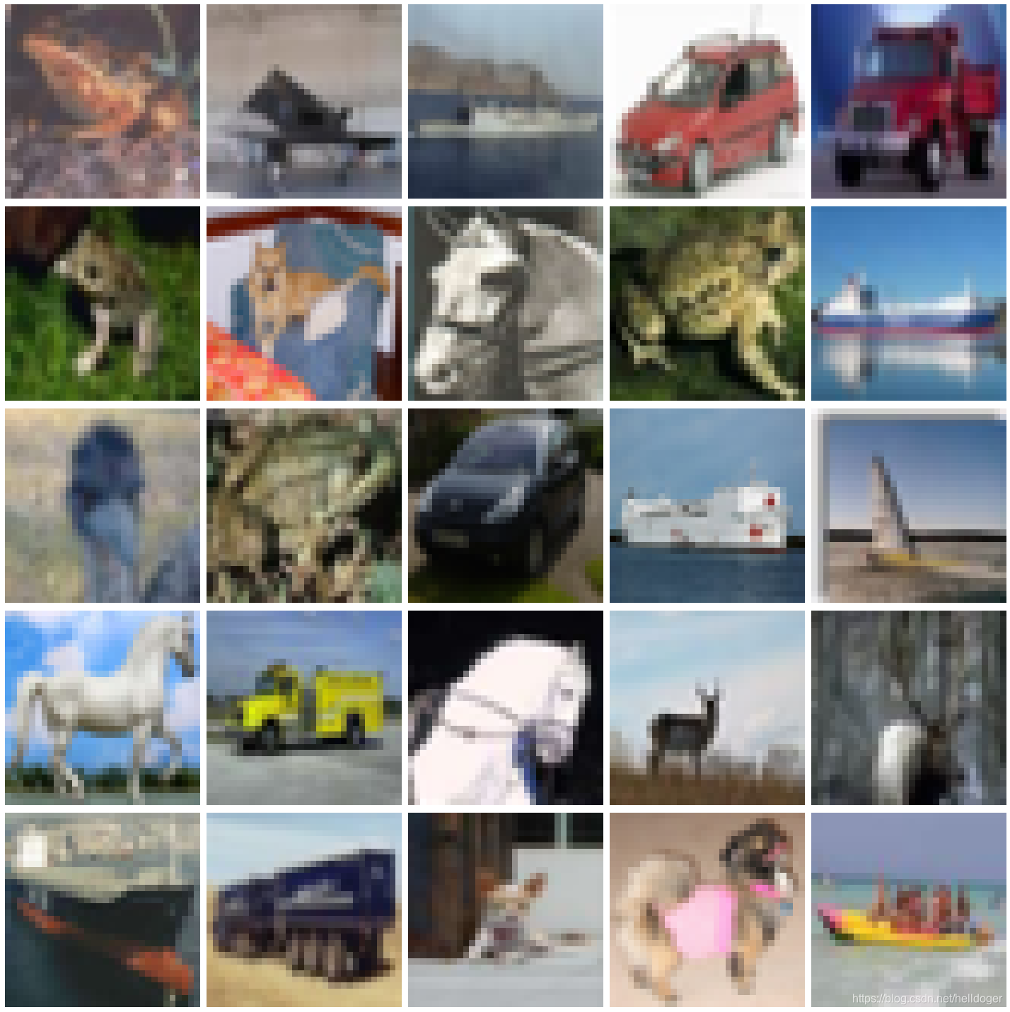
plotImages(a)
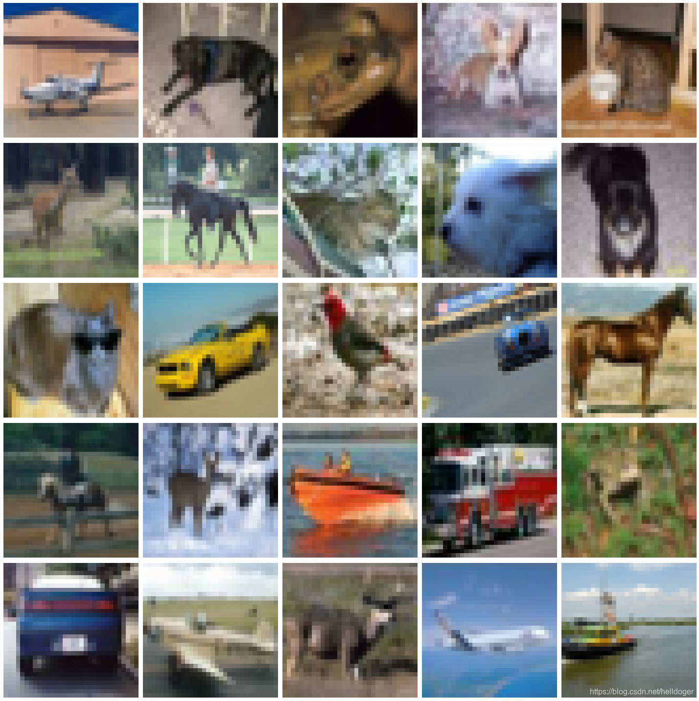
# This function will plot images in the form of a grid with 1 row and 5 columns where images are placed in each column.
def plotImages(images_arr):
    fig, axes = plt.subplots(5, 5, figsize=(20, 20))
    axes = axes.flatten()
    for img, ax in zip(images_arr, axes):
        ax.imshow(img)
        ax.axis('off')
    plt.tight_layout()
    plt.show()
plotImages(sample_training_images)
from tensorflow.keras.initializers import glorot_uniform

def Concatenate_1(X, f, filters, s = 2):

    # Retrieve Filters
    F1, F2, F3 = filters

    # Save the input value
    X_shortcut = X


    ##### MAIN PATH #####
    # First component of main path
    X = tf.keras.layers.Conv2D(F1, (1, 1), strides = (s,s),
                               padding='valid', kernel_initializer = glorot_uniform(seed=0))(X)
    X = tf.keras.layers.BatchNormalization()(X)
    X = tf.keras.layers.Activation('relu')(X)

    ### START CODE HERE ###

    # Second component of main path (≈3 lines)
    X = tf.keras.layers.Conv2D(F2, (f, f), strides = (1, 1),
                               padding='same', kernel_initializer = glorot_uniform(seed=0))(X)
    X = tf.keras.layers.BatchNormalization()(X)
    X = tf.keras.layers.Activation('relu')(X)

    # Third component of main path (≈2 lines)
    X = tf.keras.layers.Conv2D(F3, (1, 1), strides = (1, 1),
                               padding='valid', kernel_initializer = glorot_uniform(seed=0))(X)
    X = tf.keras.layers.BatchNormalization()(X)

    ##### SHORTCUT PATH #### (≈2 lines)
    X_shortcut = tf.keras.layers.Conv2D(F3, (1, 1), strides = (s, s),
                                        padding='valid', kernel_initializer = glorot_uniform(seed=0))(X_shortcut)
    X_shortcut = tf.keras.layers.BatchNormalization()(X_shortcut)

    # Final step: Add shortcut value to main path, and pass it through a RELU activation (≈2 lines)
    #X = tf.keras.layers.add([X, X_shortcut])
    X = tf.keras.layers.Concatenate()([X, X_shortcut])
    X = tf.keras.layers.Activation('relu')(X)

    ### END CODE HERE ###

    return X
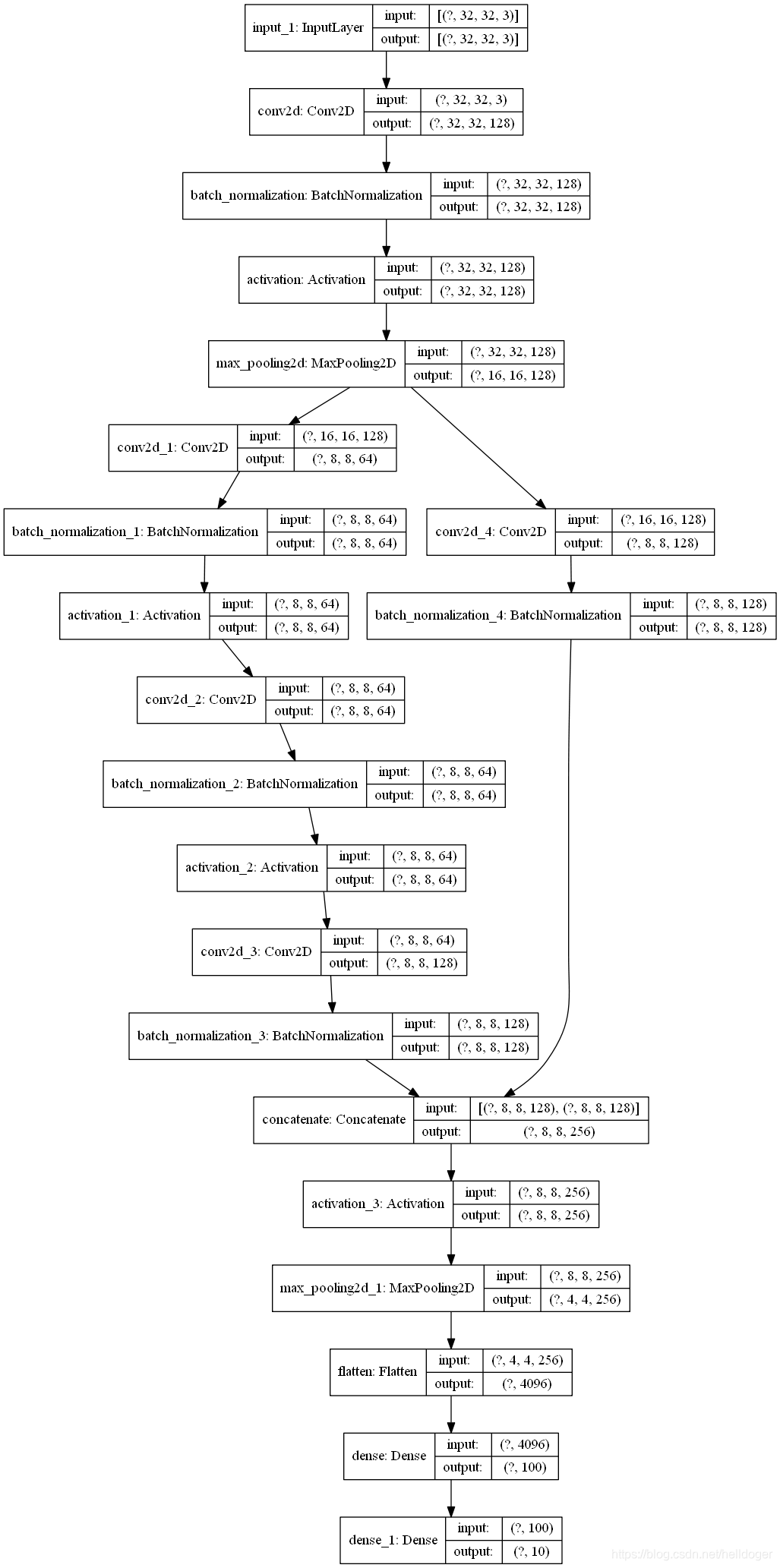
input_shape = X_train.shape[1:]
X_input = tf.keras.Input(input_shape)
X = tf.keras.layers.Conv2D(filters=128, kernel_size=(3,3), strides=(1, 1), padding='same')(X_input)
X = tf.keras.layers.BatchNormalization()(X)
X = tf.keras.layers.Activation("relu")(X)
X = tf.keras.layers.MaxPooling2D(pool_size=(2, 2), padding='valid')(X)

# Stage 2
X = Concatenate_1(X, f=3, filters=[64, 64, 128], s=2)
X = tf.keras.layers.MaxPooling2D(pool_size=(2, 2), padding='valid')(X)
#X = tf.keras.layers.Conv2D(filters=64, kernel_size=(3,3), strides=(2, 2), padding='valid')(X)
#X = tf.keras.layers.BatchNormalization()(X)
#X = tf.keras.layers.Activation("relu")(X)
X = tf.keras.layers.Flatten()(X)
X = tf.keras.layers.Dense(units=100, activation='relu')(X)
X = tf.keras.layers.Dense(units=10, activation='softmax')(X)
model = tf.keras.Model(X_input,X)
tf.keras.utils.plot_model(model,show_shapes=True)
model.compile(optimizer=tf.keras.optimizers.Adam(learning_rate=0.0005),
              loss=tf.keras.losses.CategoricalCrossentropy(from_logits=False),
              metrics=["accuracy"])
callbacks = [tf.keras.callbacks.ReduceLROnPlateau(monitor='val_loss',
                                                  patience=3,
                                                  factor=0.5,
                                                  min_lr=0.00001)]
train_iter.n,test_iter.n
(50000, 10000)
history = model.fit(x=train_iter,
                    steps_per_epoch=50000 // 32,
                    epochs=20,
                    validation_data=test_iter,
                    validation_steps=10000 // 32,
                    callbacks=callbacks)
Train for 1562 steps, validate for 312 steps
Epoch 1/20
1562/1562 [==============================] - 33s 21ms/step - loss: 2.0420 - accuracy: 0.2426 - val_loss: 21.9997 - val_accuracy: 0.1207
Epoch 2/20
1562/1562 [==============================] - 30s 19ms/step - loss: 1.8057 - accuracy: 0.3377 - val_loss: 57.0192 - val_accuracy: 0.1419
Epoch 3/20
1562/1562 [==============================] - 30s 19ms/step - loss: 1.7063 - accuracy: 0.3758 - val_loss: 119.2591 - val_accuracy: 0.1223
Epoch 4/20
1562/1562 [==============================] - 30s 19ms/step - loss: 1.6605 - accuracy: 0.3962 - val_loss: 271.0660 - val_accuracy: 0.1003
Epoch 5/20
1562/1562 [==============================] - 30s 19ms/step - loss: 1.5820 - accuracy: 0.4258 - val_loss: 329.9557 - val_accuracy: 0.1200
Epoch 6/20
1562/1562 [==============================] - 30s 19ms/step - loss: 1.5507 - accuracy: 0.4371 - val_loss: 434.2154 - val_accuracy: 0.1060
Epoch 7/20
1562/1562 [==============================] - 30s 19ms/step - loss: 1.5222 - accuracy: 0.4496 - val_loss: 394.5151 - val_accuracy: 0.1002
Epoch 8/20
1562/1562 [==============================] - 31s 20ms/step - loss: 1.4848 - accuracy: 0.4626 - val_loss: 536.6322 - val_accuracy: 0.1005
Epoch 9/20
1562/1562 [==============================] - 31s 20ms/step - loss: 1.4678 - accuracy: 0.4721 - val_loss: 521.0307 - val_accuracy: 0.1002
Epoch 10/20
1562/1562 [==============================] - 31s 20ms/step - loss: 1.4517 - accuracy: 0.4771 - val_loss: 445.1664 - val_accuracy: 0.1128
Epoch 11/20
1562/1562 [==============================] - 31s 20ms/step - loss: 1.4311 - accuracy: 0.4875 - val_loss: 505.9268 - val_accuracy: 0.1092
Epoch 12/20
1562/1562 [==============================] - 31s 20ms/step - loss: 1.4153 - accuracy: 0.4888 - val_loss: 484.1551 - val_accuracy: 0.1020
Epoch 13/20
1562/1562 [==============================] - 31s 20ms/step - loss: 1.4045 - accuracy: 0.4947 - val_loss: 475.4168 - val_accuracy: 0.1041
Epoch 14/20
1562/1562 [==============================] - 31s 20ms/step - loss: 1.3941 - accuracy: 0.5000 - val_loss: 476.9286 - val_accuracy: 0.0999
Epoch 15/20
1562/1562 [==============================] - 30s 19ms/step - loss: 1.3911 - accuracy: 0.5027 - val_loss: 400.1895 - val_accuracy: 0.1004
Epoch 16/20
1562/1562 [==============================] - 31s 20ms/step - loss: 1.3856 - accuracy: 0.5015 - val_loss: 440.0806 - val_accuracy: 0.1000
Epoch 17/20
1562/1562 [==============================] - 30s 19ms/step - loss: 1.3805 - accuracy: 0.5057 - val_loss: 407.5479 - val_accuracy: 0.1001
Epoch 18/20
 367/1562 [======>.......................] - ETA: 1:08 - loss: 1.3616 - accuracy: 0.5107
(x_train, Y_train), (x_test, Y_test) = tf.keras.datasets.cifar10.load_data()
#sample_training_images, sample_training_labels = next(ds_train.batch(batch_size = 5)) # label is one-hot coding
# This function will plot images in the form of a grid with 1 row and 5 columns where images are placed in each column.
def plotImages(images_arr):
fig, axes = plt.subplots(1, 5, figsize=(20, 20))
axes = axes.flatten()
for img, ax in zip(images_arr, axes):
ax.imshow(img)
ax.axis('off')
plt.tight_layout()
plt.show()
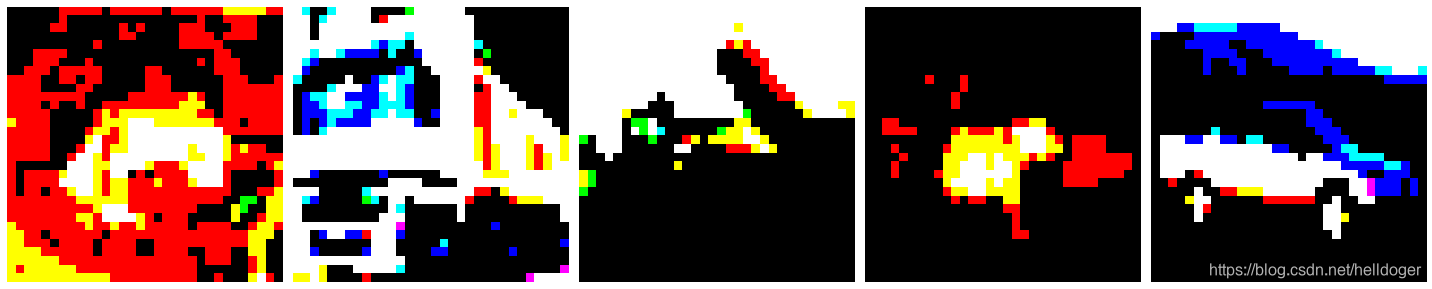
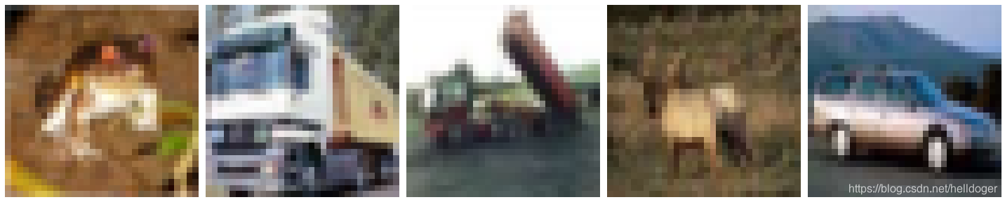
plotImages(X_train[:5]*255)
plt.show()
Clipping input data to the valid range for imshow with RGB data ([0..1] for floats or [0..255] for integers).
Clipping input data to the valid range for imshow with RGB data ([0..1] for floats or [0..255] for integers).
Clipping input data to the valid range for imshow with RGB data ([0..1] for floats or [0..255] for integers).
Clipping input data to the valid range for imshow with RGB data ([0..1] for floats or [0..255] for integers).
Clipping input data to the valid range for imshow with RGB data ([0..1] for floats or [0..255] for integers).
X_train[:5].shape
(5, 32, 32, 3)
x_train[:5].shape
(5, 32, 32, 3)
plotImages(x_train[:5])
plt.show()
import matplotlib.pyplot as plt

fig,axes = plt.subplots(2,3,subplot_kw=dict(projection='polar'),gridspec_kw=dict(left=0.1,right=0.7))
x=[1,2,3]
y=[4,5,6]
axes[0, 0].plot(x, y)
axes[1, 2].scatter(x, y)
plt.show()
[外链图片转存失败,源站可能有防盗链机制,建议将图片保存下来直接上传(img-uGSF7vUm-1590062982913)(output_30_0.png)]


 3414
3414

 被折叠的 条评论
为什么被折叠?
被折叠的 条评论
为什么被折叠?
 到【灌水乐园】发言


