


 本文介绍了VizPool,一个用于Python的数据可视化库,它提供了丰富的图表类型,如饼图、箱线图、直方图等,同时展示了如何结合VizPool和sklearn进行数据探索、特征工程和模型训练,包括使用LogisticRegression、RandomForestClassifier等进行模型评估。
VizPool,一个超强的Python可视化库!
相关文档地址如下
https://github.com/Hassi34/VizPool
https://jovian.ai/hasnainmehmood3435/vizpool-static-api
可以使用pip安装使用。
pip install vizpool -i https://mirror.baidu.com/pypi/simple
安装好以后,导入相关库。
import vizpool as vizpool
from vizpool.static import EDA
from vizpool.static import Evaluation
import seaborn as sns
import pandas as pd
from sklearn.model_selection import train_test_split
from sklearn.linear_model import LogisticRegression, SGDClassifier, LinearRegression
from sklearn.svm import SVC
from sklearn.tree import ExtraTreeClassifier
from sklearn.compose import ColumnTransformer
from sklearn.pipeline import Pipeline
from sklearn.preprocessing import StandardScaler, OneHotEncoder
from sklearn.ensemble import RandomForestClassifier
from sklearn.metrics import accuracy_score
from sklearn.preprocessing import LabelEncoder
# 加载数据集
df = pd.read_csv(“tips.csv”)
# EDA实例化(Exploratory Data Analysis)
tips_eda = EDA(df)
加载数据,进行数据探索分析工作。
其中tips.csv可以在【GitHub】上获取。
https://github.com/mwaskom/seaborn-data/blob/master/tips.csv

其中数据含义如下。
total_bill:消费总金额
tip:小费金额
sex:性别
smoker:是否吸烟
day:消费日期
time:消费时段
size:聚餐人数
下面就来看看图表示例吧。
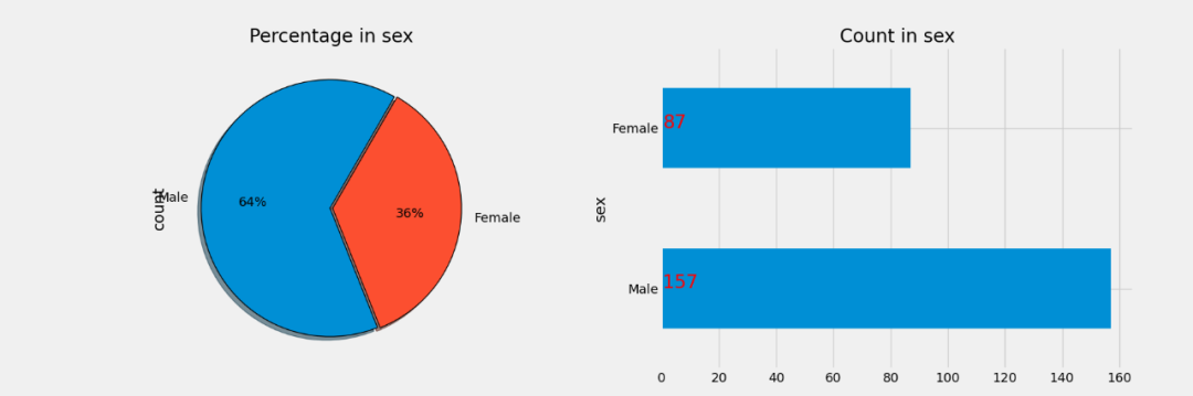
01. 饼图条形图
# 饼图条形图
plt = tips_eda.pie_bar(hue=‘sex’);
plt.savefig(“Pie_bar.png”)
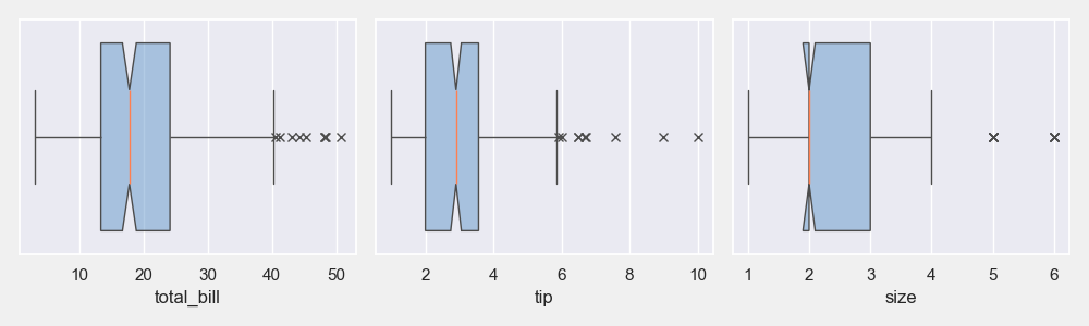
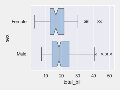
02. 箱线图
# 所有数值列的箱线图网格
plt = tips_eda.boxplot(height=3, width=10)
plt.savefig(“Box_all.png”)
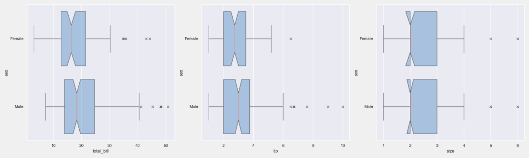
# 指定分类的所有数值列的箱线图网格
plt = tips_eda.boxplot(hue=‘sex’, height=6)
plt.savefig(“Box_sex.png”)
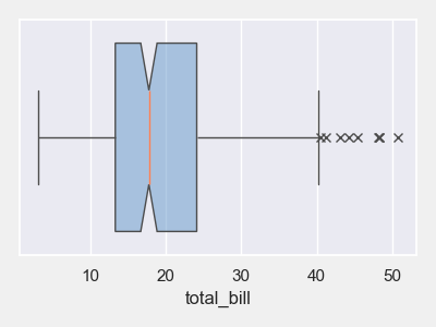
# 特定数值列的箱线图
plt = tips_eda.boxplot(col_to_plot=[‘total_bill’], width=4, height=3)
plt.savefig(“Box_total_bill.png”)
# 指定分类的任何数值的箱线图
plt = tips_eda.boxplot(col_to_plot=[‘total_bill’], hue=‘sex’, width=4, height=3)
plt.savefig(“Box_sex_total_bill.png”)
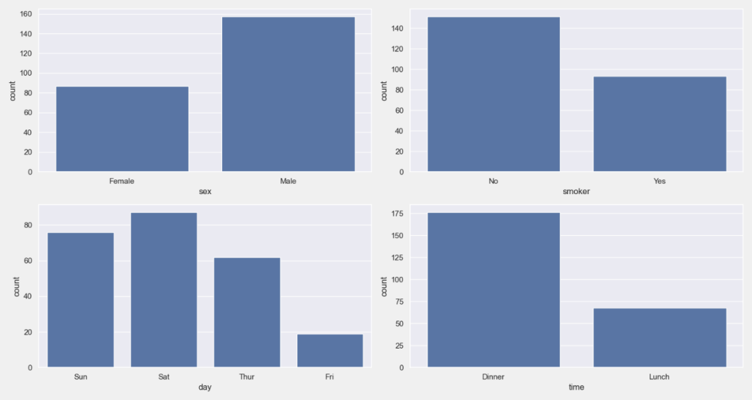
03. 计数图
# 数据中所有非数字列的计数图网格
plt = tips_eda.countplot()
plt.savefig(“Count.png”)
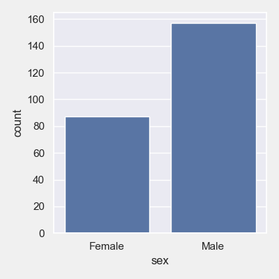
# 单个分类列的计数图
plt = tips_eda.countplot([‘sex’], height=4, width=4)
plt.savefig(“Count_sex.png”)
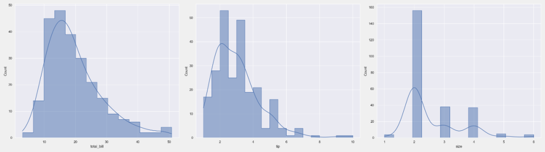
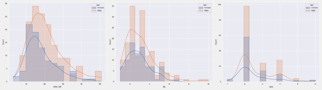
04. 直方图
# 所有数值列的直方图网格
plt = tips_eda.histogram(height=7)
plt.savefig(“Histogram.png”)
# 直方图, 其中分类列作为关键字参数传递给hue
plt = tips_eda.histogram(hue=‘sex’, height=7)
plt.savefig(“Histogram_sex.png”)
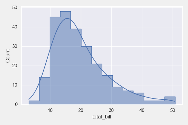
# 特定数值列的直方图
plt = tips_eda.histogram(col_to_plot=[‘total_bill’], height=4, width=6)
plt.savefig(“Histogram_total_bill.png”)
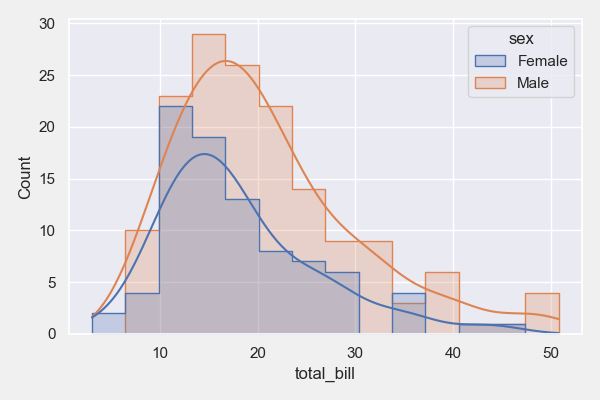
# 指定分类的特定数值列的直方图
plt = tips_eda.histogram(col_to_plot=[‘total_bill’], hue=‘sex’, height=4, width=6)
plt.savefig(“Histogram_sex_total_bill.png”)
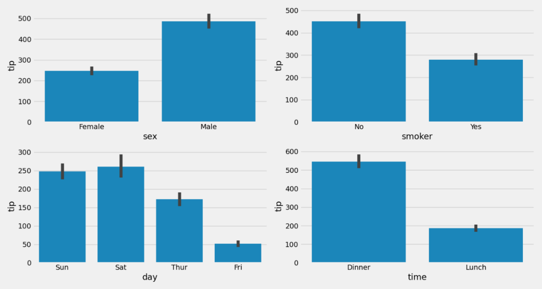
05. 柱状图
# 所有分类列相对于所提供的数字列的条形图网格
plt = tips_eda.barplot(y=‘tip’, estimator=‘sum’)
plt.savefig(“Bar.png”)
# 针对所提供的数字列的所有分类列的条形图网格,色调设置为分类列
plt = tips_eda.barplot(y=‘tip’, hue=‘time’).show()
plt.savefig(“Bar_time.png”)
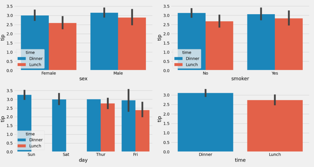
# 选取单变量的柱状图
plt = tips_eda.barplot(y=‘tip’, col_to_plot=‘smoker’, hue=‘time’, height=3, width=4)
plt.savefig(“Bar_single.png”)

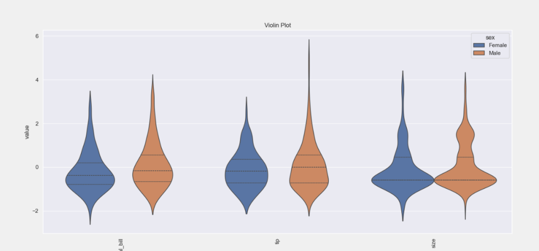
06. 小提琴图
# 针对目标列或分类列的所有数值列的Violinplot作为关键字参数传递
plt = tips_eda.violinplot(hue=‘sex’, height=7)
plt.savefig(“Violin.png”)
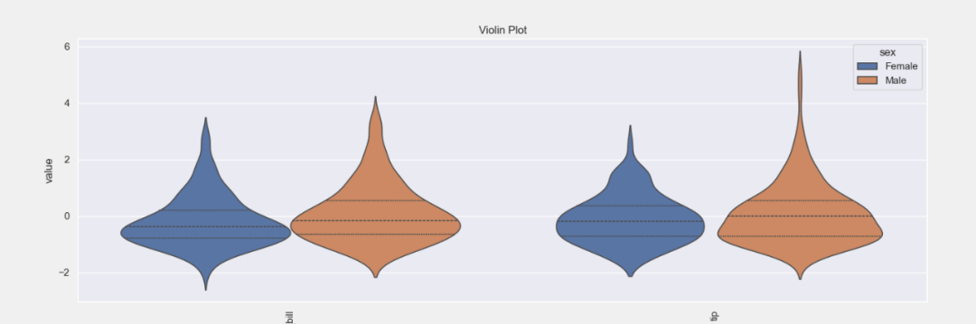
# 作为关键字参数传递的针对目标列或分类列的选择性数值列的Violinplot
plt = tips_eda.violinplot(col_to_plot=[‘total_bill’, ‘tip’], hue=‘sex’, height=5)
plt.savefig(“Violin_col.png”)
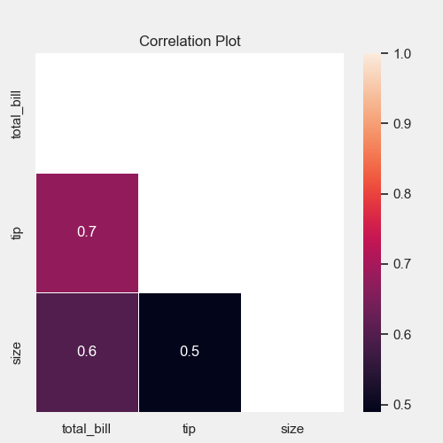
07. 热力图
# 热力图
plt = tips_eda.corr_heatmap(height=5, width=5)
plt.savefig(“Correlation_Heatmap.png”)
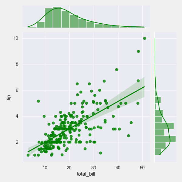
08. 联合图
# 两个数值变量的联合图
plt = tips_eda.jointplot(x=‘total_bill’,
y=‘tip’,
height=5, width=5,
color=‘green’)
plt.savefig(“Joint.png”)
09. 特征图
# 包含作为关键字参数传递的分类列的所有数值特征的成对图
plt = tips_eda.pairplot(hue=‘sex’, height=5, width=8)
plt.savefig(“Pair.png”)

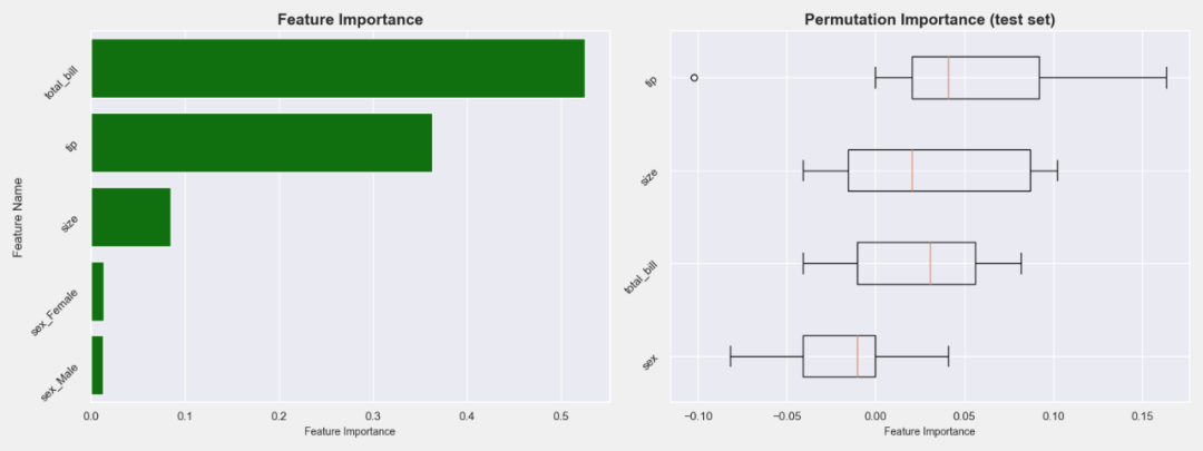
10. 模型训练和评估
选择列数据, 并尝试预测这个人是否吸烟。
# 使用sklearn机器学习管道获取特征重要性
pipeline_data = df[[“total_bill”, “tip”, “size”, “sex”, “smoker”]]
target_class_labels = pipeline_data[‘smoker’].unique().tolist()
target = LabelEncoder().fit_transform(pipeline_data.pop(‘smoker’))
X_train, X_val, y_train, y_val = train_test_split(pipeline_data, target, test_size=0.2, random_state=42)
# 实例化评估类
model_eval = Evaluation(y_val)
col_trans = ColumnTransformer(transformers=[
(‘num_processing’, StandardScaler(), [“total_bill”, “tip”, “size”]),
(‘cat_processing’, OneHotEncoder(), [‘sex’])
], remainder=‘drop’)
pipe_rfc = Pipeline(steps=[
(‘tranformer’, col_trans),
(‘classifier’, RandomForestClassifier())
])
pipe_rfc.fit(X_train, y_train)
plt = model_eval.feature_importance(pipe_rfc, X_val=X_val, pipeline=True,
height=6, width=16)
plt.savefig(“RandomForestClassifier.png”)
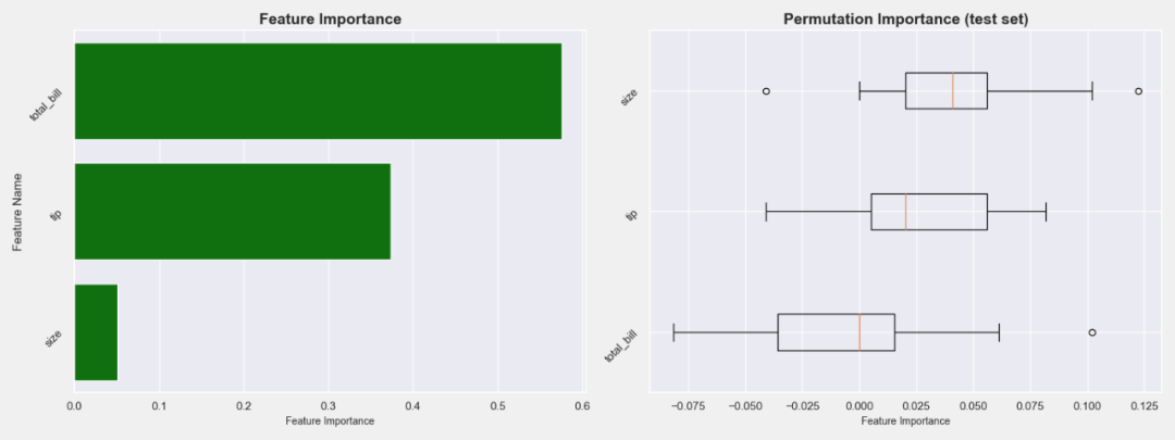
# 用估计器获得特征的重要性
df = df[[“total_bill”, “tip”, “size”, “smoker”]]
target_class_labels = df[‘smoker’].unique().tolist()
target = LabelEncoder().fit_transform(df.pop(‘smoker’))
X_train, X_val, y_train, y_val = train_test_split(df, target, test_size=0.2, random_state=42)
X_train.shape, X_val.shape, y_train.shape, y_val.shape
logistic_reg_clf = LogisticRegression()
logistic_reg_clf.fit(X_train, y_train)
logistic_predictions = logistic_reg_clf.predict(X_val)
etc = ExtraTreeClassifier()
etc.fit(X_train, y_train)
etc_predictions = etc.predict(X_val)
svc = SVC(probability=True)
svc.fit(X_train, y_train)
svc_predictions = svc.predict(X_val)
sgd = SGDClassifier()
sgd.fit(X_train, y_train)
sgd_predictions = sgd.predict(X_val)
plt = model_eval.feature_importance(etc, X_val=X_val,
height=6, width=16)
plt.savefig(“ExtraTreeClassifier.png”)
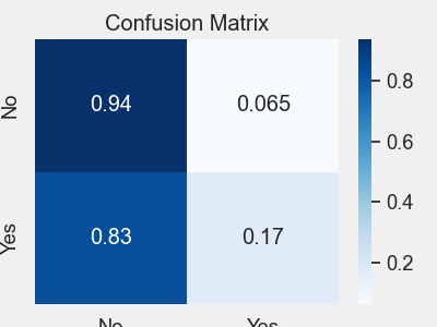
# 带比率的混淆矩阵
plt = model_eval.confusion_matrix(logistic_predictions,
target_names=target_class_labels,
height=3, width=4)
plt.savefig(“predictions_rate.png”)
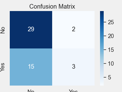
# 带计数的混淆矩阵
plt = model_eval.confusion_matrix(logistic_predictions, target_names=target_class_labels,
height=3, width=4, normalize=False)
plt.savefig(“predictions_count.png”)
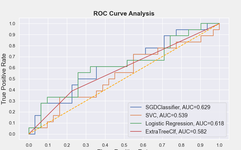
# ROC曲线
plt = model_eval.auc_roc_plot(X_val, [sgd, svc, logistic_reg_clf, etc],
[‘SGDClassifier’, ‘SVC’, ‘Logistic Regression’, ‘ExtraTreeClf’],
height=5, width=8)
plt.savefig(“ROC.png”)
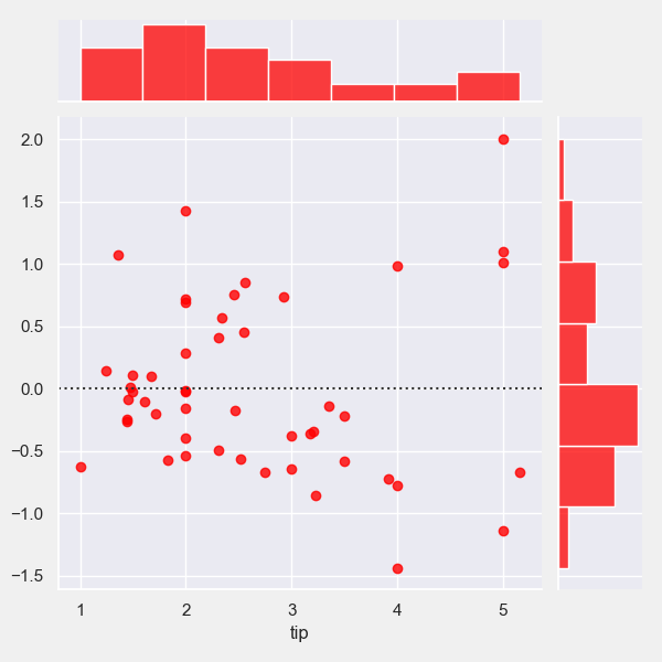
# 残差图
# 训练线性回归模型
lr = LinearRegression()
X = df[[‘size’, ‘total_bill’]]
y = df[‘tip’]
X_train, X_val, y_train, y_val = train_test_split(X, y, test_size=0.2, random_state=42)
lr.fit(X_train, y_train)
y_predicted = lr.predict(X_val)
# 模型评估
lr_model_eval = Evaluation(y_val)
plt = lr_model_eval.residplot(y_predicted=y_predicted, color=‘red’)
plt.savefig(“predicted.png”)


 到【灌水乐园】发言


