概率论与随机过程笔记（2）：离散随机变量（1）

概率论与随机过程笔记（2）：离散随机变量（1）

2019-11-25

---

*这部分的笔记依据Dimitri P. Bertsekas和John N. Tsitsiklis的《概率导论》第2章前半部分的内容。

2.1 关于离散随机变量的几个概念

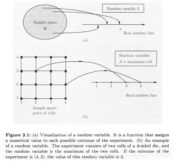
Given an experiment and the corresponding set of possible outcornes (the sample space), a random variable associates a particular number with each outcome: see Fig. 2.1. We refer to this number as the numerical value or simply the value of the random variable. mathematically, a random variable is a real-valued function of the experimental outcome.

Main Concepts Related to Random Variables:

Starting with a probabilistic model of an experiment:

• A random variable is a real-valued function of the outcome of the experiment.
• A function of a random variable defines another random variable.
• We can associate with each random variable certain “averages” of interest, such as the mean and the variance.
• A random variable can be conditioned on an event or on another random variable.
• There is a notion of independence of a random variable from an event or from another random variable.

A random variable is called discrete if its range (the set of values that it can take) is either finite or countably infinite. A random variable that can take an uncountably infinite number of values is not discrete.

Concepts Related to Discrete Random Variables

Starting with a probabilistic model of an experiment:

• A discrete random variable is a real-valued function of the outcome of the experiment that can take a finite or countably infinite number of values.
• A discrete random variable has an associated probability mass funcion (PMF), which gives the probability of each numeric the random variable can take.
• A function of a discrete random variable defines another discrete random variable, whose PMF can be obtained from the PMF of the original random variable.

2.2 概率质量函数（probability mass function）

The most important way to characterize a random variable is through the probabilities of the values that it can take. For a discrete random variable $X$, these are captured by the probability mass function (PMF for short) of $X$, denoted $p_X$. In particular. if x is any possible value of $X$. the probability mass of $x$. lenoted $p_X(x)$. is the probability of the event { X = x } \{X = x\} { X=x} consisting of: that give rise to a value of $X$ equal to $x$: p X ( x ) = P ( { X = x } ) p_X(x) = P(\{X=x\}) pX​(x)=P({ X=x})

We will use upper case characters ($X$) to denote random variables, and lower case characters ($x$) to denote real numbers such as the numerical values of a random variable. Note that $$\sum _x{p}_X(x)=1$$

Calculation of the PMF of a Random Variable $X$

For each possible value $x$ of $X$:

• collect all the posible outcomes that give rise to the event { X = x } \{X=x\} { X=x}
• add their probabilities to obtain $p_X(x)$

By a similar argument, for any set $S$ of possible values of $X$,we have $$P(x\in S)=\sum _{x\in S}{p}_X(x)$$

【伯努利随机变量（The Bernoulli Random Variable）】Consider the toss of a coin, which comes up a head with probability $p$, and a tail with probability $1-p$. The Bernoulli random variable takes the two values 1 and 0, depending on whether the outcome is a head or a tail:
$$f(x)=\{\begin{array}{ll}1& \text{if a head}\\ 0& \text{if a tail}\end{array}$$ Its PMF is
$$f(x)=\{\begin{array}{ll}p& \text{if k=1}\\ 1-p& \text{if k=0}\end{array}$$
For all its simplicity. the Bernoulli random variable is very important. In practice. it is used to model generic probabilistic situations with just two outcomes.

【二项随机变量（The Binomial Random Variable）】A coin is tossed n times. At each toss, the coin comes up a head with probability $p$, and a tail with probability $1-p$, independent of prior tosses. Let $X$ be the number of heads in the $n$-toss sequence. We refer to $X$ as a binomial random variable with parameters $n$ and $p$. PMF of $X$ consists of the binomial probabilities that were calculated
$$p_X(k)=P(x=K)=\left(\genfrac{}{}{0ex}{}{n}{k}\right)p^k(1$$