初识机器学习 | 4.线性回归

import pandas as pd
import numpy as np
import matplotlib.pyplot as plt

%matplotlib
%matplotlib inline
%config InlineBackend.figure_format = 'retina'

Using matplotlib backend: MacOSX

简单线性回归的实现

只有一个样本特征, 及只有一个变量： y = kx + b

最优化损失函数：

$$\sum _{i=1}^m{\left(y^{(i)}-a{x}^{(i)}-b\right)}^2$$

使用最小二乘法问题: 最小化误差的平方

$$\{\begin{array}{l}a=\frac{{\sum }_{i=1}^m\left(x^{(i)}-\bar{x}\right)\left(y^{(i)}-\bar{y}\right)}{{\sum }_{i=1}^m{\left(x^{(i)}-\bar{x}\right)}^2}\\ \hat{b}=\bar{y}-a\bar{x}\end{array}$$

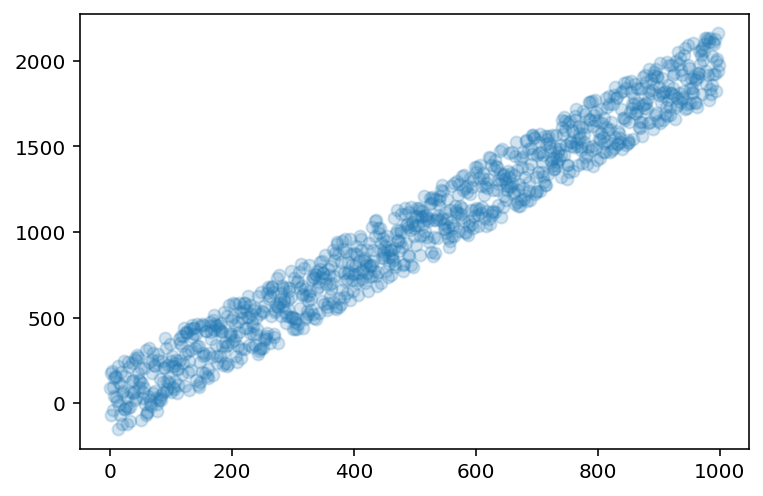
SIZE = 1000
UNDULATE = 200

x = np.arange(SIZE)
y = x * 2 + np.random.randint(-UNDULATE, UNDULATE, size=SIZE)

plt.scatter(x, y, alpha=0.2)
plt.show()

线性回归实现

class SimpleLinearRegression():
    """ 简单线性会回归 """
    def __init__(self):
        self.a = 0
        self.b = 0
    
    def fit(self, x, y):
        x_avg = x.mean()
        y_avg = y.mean()

        molecule = 0
        for x_item, y_item in zip(x, y):
            molecule += (x_item-x_avg) * (y_item-y_avg)

        denominator = 0
        for item in x:
            denominator += pow((item-x_avg), 2)

        self.a = molecule / denominator
        self.b = y_avg - self.a * x_avg

    def predict(self, x):
        return x * self.a + self.b    

obj =  SimpleLinearRegression()
%time obj.fit(x, y)
y_predict = obj.predict(x)

print('a=', obj.a)
print('b=', obj.b)

plt.scatter(x, y, alpha=0.2)
plt.plot(x, y_predict, color='r')
plt.show()

CPU times: user 11.9 ms, sys: 2.54 ms, total: 14.5 ms
Wall time: 14.5 ms
a= 1.988647556647557
b= 6.512545454545261

使用向量计算优化

使用向量计算，避免走循环计算。可以大幅度提高效率。

class SimpleLinearRegression2():
    """ 简单线性会回归(向量实现) """    
    def __init__(self):
        self.a = 0
        self.b = 0
    
    def fit(self, x, y):
        x_avg = x.mean()
        y_avg = y.mean()

        molecule = np.dot(x-x_avg, y-y_avg)
        denominator = np.dot(x-x_avg, x-x_avg)

        self.a = molecule / denominator
        self.b = y_avg - self.a * x_avg

    def predict(self, x):
        return x * self.a + self.b    

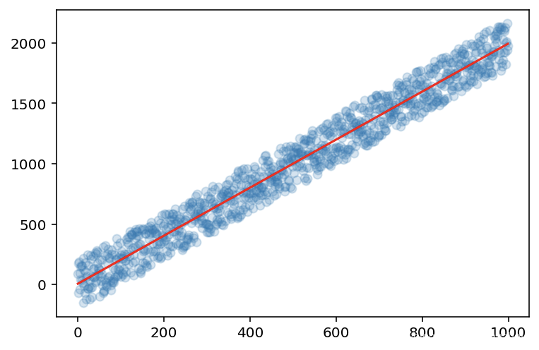
obj =  SimpleLinearRegression2()
%time obj.fit(x, y)
y_predict = obj.predict(x)

print('a=', obj.a)
print('b=', obj.b)

plt.scatter(x, y, alpha=0.2)
plt.plot(x, y_predict, color='r')
plt.show()

CPU times: user 180 µs, sys: 20 µs, total: 200 µs
Wall time: 225 µs
a= 1.988647556647557
b= 6.512545454545261

模型评价

MSE

$$\frac{1}{m}\sum _{i=1}^m{\left(y_{test}^{(i)}-{\hat{y}}_{test}^{(i)}\right)}^2$$

np.dot(y_predict - y, y_predict - y) / len(y)

12879.24321590063

RMSE

$$\sqrt{\frac{1}{m}\sum _{i=1}^m{\left(y_{\text{tare }}^{(10)}-{\dot{y}}_{\text{irst }}^{(i)}\right)}^2}=\sqrt{MS{E}_{\text{tert }}}$$

import math
math.sqrt(np.dot(y_predict - y, y_predict - y) / len(y))

113.48675348207222

MAE

$$\frac{1}{m}\sum _{i=1}^m\left|y_{test}^{(i)}-{\hat{y}}_{test}^{(i)}\right|$$

np.sum(np.absolute(y-y_predict)) / len(y)

97.3878859088179

R Square

$$1-\frac{MSE(\hat{y},y)}{\mathrm{Var}(y)}$$

1 - np.dot(y_predict - y, y_predict - y)/len(y)/np.var(y) 

0.9623896540119193

多元线性回归

使目标函数尽可能小:
$$\sum _{i=1}^m{\left(y^{(i)}-{\hat{y}}^{(i)}\right)}^2$$

$$\{\begin{array}{l}{X}_0^{(i)}=1\\ {\hat{y}}^{(i)}={\theta }_0{X}_0^{(i)}+{\theta }_1{X}_1^{(i)}+{\theta }_2{X}_2^{(i)}+\dots +{\theta }_n{X}_n^{(i)}\end{array}$$

=>

$$\{\begin{array}{l}\theta ={\left({\theta }_0,{\theta }_1,{\theta }_2,\dots ,{\theta }_n\right)}^T\\ {\hat{X}}^{(i)}=\left(X_0^{(i)},X_1^{(i)},X_2^{(i)},\dots ,X_n^{(i)}\right)\\ {\hat{y}}^{(i)}=X^{(i)}\cdot \theta \end{array}$$

=>

$$X_b=\left(\begin{array}{ccccc}1& X_1^{(1)}& X_2^{(1)}& \dots & X_n^{(1)}\\ 1& X_1^{(2)}& X_2^{(2)}& \dots & X_n^{(2)}\\ \dots & & & & \dots \\ 1& X_1^{(m)}& X_2^{(m)}& \dots & X_n^{(m)}\end{array}\right)\theta =\left(\begin{array}{c}{\theta }_0\\ {\theta }_1\\ {\theta }_2\\ \dots \\ {\theta }_n\end{array}\right)$$

$$\hat{y}=X_b\cdot \theta$$

=> 最终推导出(多元线性回归的正规方程解(Normal Euqation))

$$\begin{gathered} \theta ={\left(X_b^T{X}_b\right)}^{-1}{X}_b^{T}y \\ \hat{y}=X_b\cdot \theta \end{gathered}$$

• 优点: 不需要对数据做归一化处理
• 缺点: 时间复杂度高 O(n^3) 优化到O(n^2.4)

class CustomLinearRegression():
    """线性回归 """
    def __init__(self):
        self._theta = None
        # 截距
        self.intercept = None
        # 参数系数
        self.coef = None
    
    def fit(self, x_train, y_train):
        # 矩阵第一列填充1
        X_b = np.hstack([np.ones((len(train_x_df),1)), train_x_df])
        # np.linalg.inv求逆矩阵
        self._theta = np.linalg.inv(np.dot(X_b.T,X_b)).dot(X_b.T).dot(y_train)
        self.intercept = self._theta[0]
        self.coef = self._theta[1:]        
        
        return self
        
    def predict(self, x_predict):
        X_b = np.hstack([np.ones((len(train_x_df),1)), train_x_df])
        return np.dot(X_b, self._theta)
    
    def score(self, y, y_predict):
        """ """
        return 1 - np.dot(y_predict - y, y_predict - y)/len(y)/np.var(y) 

# 使用波士顿房价数据测试
from sklearn import datasets
from sklearn.linear_model import LinearRegression

# 加载数据
boston = datasets.load_boston()
train_x_df = boston['data']
train_y_df = boston['target']

estimator = CustomLinearRegression()
estimator.fit(train_x_df, train_y_df)
predit_y_df = estimator.predict(train_x_df)
print('---- CustomLinerRegression ----')
print('intercept: ', estimator.intercept)
print('coef: ', estimator.coef)
print('score:', estimator.score(train_y_df, predit_y_df))

estimator = LinearRegression()
estimator.fit(train_x_df, train_y_df)
predit_y_df = estimator.predict(train_x_df)
print('\n---- SkleanLinerRegression ----')
print('intercept: ', estimator.intercept_)
print('coef: ', estimator.coef_)
print('score:', estimator.score(train_x_df, train_y_df))

---- CustomLinerRegression ----
intercept:  36.45948838506836
coef:  [-1.08011358e-01  4.64204584e-02  2.05586264e-02  2.68673382e+00
 -1.77666112e+01  3.80986521e+00  6.92224640e-04 -1.47556685e+00
  3.06049479e-01 -1.23345939e-02 -9.52747232e-01  9.31168327e-03
 -5.24758378e-01]
score: 0.7406426641094095

---- SkleanLinerRegression ----
intercept:  36.459488385090125
coef:  [-1.08011358e-01  4.64204584e-02  2.05586264e-02  2.68673382e+00
 -1.77666112e+01  3.80986521e+00  6.92224640e-04 -1.47556685e+00
  3.06049479e-01 -1.23345939e-02 -9.52747232e-01  9.31168327e-03
 -5.24758378e-01]
score: 0.7406426641094095

自定义实现的线性回归算法与sklean关键几个参数值一样。同时线性回归学习到的参数值对数据具有较强的解释性.

较强的解释性

线性回归学习到的参数值对数据具有较强的解释性.

print(boston.DESCR)

.. _boston_dataset:

Boston house prices dataset
---------------------------

**Data Set Characteristics:**  

    :Number of Instances: 506 

    :Number of Attributes: 13 numeric/categorical predictive. Median Value (attribute 14) is usually the target.

    :Attribute Information (in order):
        - CRIM     per capita crime rate by town
        - ZN       proportion of residential land zoned for lots over 25,000 sq.ft.
        - INDUS    proportion of non-retail business acres per town
        - CHAS     Charles River dummy variable (= 1 if tract bounds river; 0 otherwise)
        - NOX      nitric oxides concentration (parts per 10 million)
        - RM       average number of rooms per dwelling
        - AGE      proportion of owner-occupied units built prior to 1940
        - DIS      weighted distances to five Boston employment centres
        - RAD      index of accessibility to radial highways
        - TAX      full-value property-tax rate per $10,000
        - PTRATIO  pupil-teacher ratio by town
        - B        1000(Bk - 0.63)^2 where Bk is the proportion of blacks by town
        - LSTAT    % lower status of the population
        - MEDV     Median value of owner-occupied homes in $1000's

    :Missing Attribute Values: None

    :Creator: Harrison, D. and Rubinfeld, D.L.

This is a copy of UCI ML housing dataset.
https://archive.ics.uci.edu/ml/machine-learning-databases/housing/


This dataset was taken from the StatLib library which is maintained at Carnegie Mellon University.

The Boston house-price data of Harrison, D. and Rubinfeld, D.L. 'Hedonic
prices and the demand for clean air', J. Environ. Economics & Management,
vol.5, 81-102, 1978.   Used in Belsley, Kuh & Welsch, 'Regression diagnostics
...', Wiley, 1980.   N.B. Various transformations are used in the table on
pages 244-261 of the latter.

The Boston house-price data has been used in many machine learning papers that address regression
problems.   
     
.. topic:: References

   - Belsley, Kuh & Welsch, 'Regression diagnostics: Identifying Influential Data and Sources of Collinearity', Wiley, 1980. 244-261.
   - Quinlan,R. (1993). Combining Instance-Based and Model-Based Learning. In Proceedings on the Tenth International Conference of Machine Learning, 236-243, University of Massachusetts, Amherst. Morgan Kaufmann.

df = pd.DataFrame({
    'feature': boston['feature_names'][np.argsort(estimator.coef_)],
    'value':estimator.coef_[np.argsort(estimator.coef_)]
})
df

	feature	value
0	NOX	-17.766611
1	DIS	-1.475567
2	PTRATIO	-0.952747
3	LSTAT	-0.524758
4	CRIM	-0.108011
5	TAX	-0.012335
6	AGE	0.000692
7	B	0.009312
8	INDUS	0.020559
9	ZN	0.046420
10	RAD	0.306049
11	CHAS	2.686734
12	RM	3.809865

根据学习到的参数可以发现:

• 正相关最大值为RM(房间个数)，即房间数越大,房价越贵，且正相关性最强。
• 负相关最大值NOX(一氧化氮浓度)，即NOX越大,房价越便宜，且负相关性最强。