


 本文提出了一种预训练图神经网络的方法,旨在提取图结构的通用特征,无需标签信息。通过三种结构相关的预训练任务,包括去噪连接重建、中心得分排名和聚类,模型能够学习到从局部到全局的结构信息。实验证明,预训练的模型在各种下游任务中表现出色,尤其是在节点分类、链路预测和图形分类等任务中。
Paper : Pre-Training Graph Neural Networks for Generic Structural Feature Extraction
Code :
摘要
作者想要解决的任务是根据图结构进行预测,通过构造三种与图结构相关的损失函数——去噪连接重建、中心得分排名、集群,作者给出的预训练算法得到的模型参数可以包含从图的局部到全局不同层次的结构信息。由于没有标签的要求,只是对结构信息进行预训练,因此可以应用到比较大的数据集上去,可以downstream 到少标签的任务中。
算法
算法的整体框架如下所示
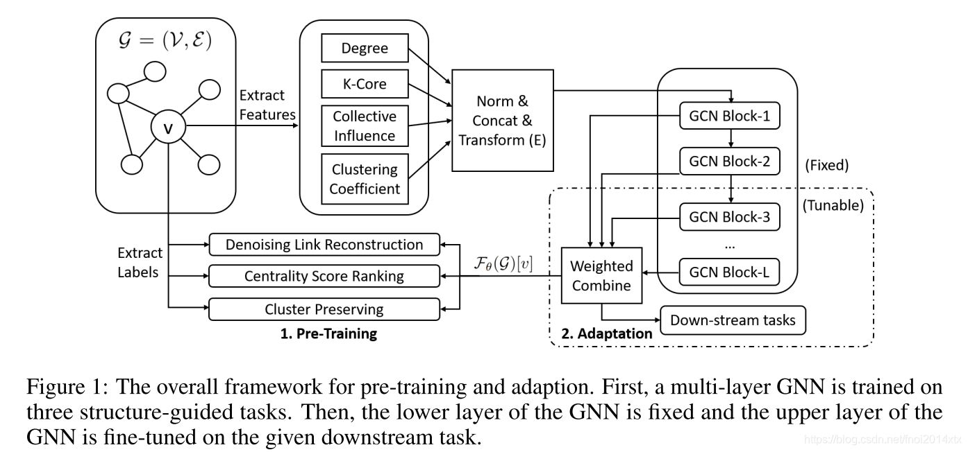
作者提出的算法主要针对网络的结构信息进行pretrain,在不同的任务中,只有网络的结构信息具有通用性,希望初始化的参数可以容纳足够结构信息。算法的流程大致如下所示
- 对图结构中的节点提取出4种结构信息,为了应对不同规模的图需要对部分特征进行正则化
- 将正则化后的信息连接起来,使用Encoder映射到 R d \mathbb R^d Rd 的空间中,其中 d d d 为预训练网络的输入特征维度
- 搭建多层GCN网络,将不同层的点特征输出连接起来进行预测
- 针对3种从局部到整体的图结构相关的任务进行训练
当网络得到充分训练时,GCN的参数包含了较为丰富的网络结构信息,作为GCN模型的初始化参数进行down-stream task 的finetune。
节点处定义的四种结构信息定义如下
- 度数:定义了节点的局部重要性
- 核数:定义了节点的局部连接情况,如果一个点的核数为K,表示存在一个子图包含该点,子图中点度数的最小值是K
- CI:定义了节点的邻居的重要性,其中
C
I
L
(
v
)
CI_{L}(v)
CIL(v) 定义为
C I L ( v ) = ( D e g ( v ) − 1 ) ∑ u ∈ N ( v , L ) ( D e g ( u ) − 1 ) CI_L(v) = (Deg(v)-1)\sum_{u\in N(v,L)}(Deg(u)-1) CIL(v)=(Deg(v)−1)u∈N(v,L)∑(Deg(u)−1)
其中 N ( v , L ) N(v,L) N(v,L) 表示节点 v v v 的 L-hop 邻居 - CC:在节点
v
v
v 其1跳邻域内包含v的所有三元组中,封闭三元组的比例
C C ( v ) = 2 Triangle ( v ) D e g ( v ) ( D e g ( v ) − 1 ) CC(v) = \frac{2\text{Triangle}(v)}{Deg(v)(Deg(v)-1)} CC(v)=Deg(v)(Deg(v)−1)2Triangle(v)
使用Min-Max方法对它们进行正则化,经过一个Encoder之后点的结构特征被映射到了 R d \mathbb R^d Rd 上,GNN的结构定义为
H ( l + 1 ) = σ ( D ~ − 1 2 A ~ D ~ − 1 2 norm ( σ ( H ( l ) W 1 ( l ) ) W 2 ( l ) ) ) H^{(l+1)} = \sigma(\widetilde D^{-\frac{1}{2}}\widetilde A\widetilde D^{-\frac{1}{2}}\text{norm}(\sigma (H^{(l)}W_1^{(l)})W_2^{(l)})) H(l+1)=σ(D −21A D −21norm(σ(H(l)W1(l))W2(l)))
使用不同层的点特征矩阵进行加权求和,表示GNN的输出
F task = α task ∑ l = 1 L β l task H l where β l task = exp ( ϕ l task ) ∑ l = 1 L exp ( ϕ l task ) \\ F^{\text{task}} = \alpha^\text{task} \sum_{l=1}^L \beta_l^\text{task} H^l \\\text{where } \beta^\text{task}_l = \frac{\exp(\phi_l^\text{task})}{\sum_{l=1}^L \exp(\phi_l^\text{task})} Ftask=αtaskl=1∑LβltaskHlwhere βltask=∑l=1Lexp(ϕltask)exp(ϕltask)
与结构相关的优化任务有3种,分别是
-
去噪的边连接重建:随机移除邻接矩阵中的边,然后根据加了噪声的邻接矩阵预测原始邻接矩阵。定义pairwise decoder D rec ( ⋅ , ⋅ ) D^\text{rec}(\cdot,\cdot) Drec(⋅,⋅),预测节点 u , v u,v u,v 之间是否连边,即 A ^ u , v = D rec ( F rec ( u ) , F rec ( v ) ) \widehat A_{u,v} = D^\text{rec}(F^\text{rec}(u),F^\text{rec}(v)) A u,v=Drec(Frec(u),Frec(v)),损失函数定义为
L rec = − ∑ u , v ∈ V ( A u , v log A ^ u , v + ( 1 − A u , v ) log ( 1 − A ^ u , v ) ) \mathcal L_\text{rec} = -\sum_{u,v\in V}(A_{u,v}\log \widehat A_{u,v}+(1-A_{u,v})\log (1-\widehat A_{u,v})) Lrec=−u,v∈V∑(Au,vlogA u,v+(1−Au,v)log(1−A u,v)) -
中心分数排序:点中心性衡量了在整个图中节点的重要性,使用GNN来预测点中心分数的排序。有以下四种点中心性分数
- Eigencentrality :
Eigenvector centrality of a node v is calculated based on the centrality of its neighbors. The eigenvector centrality for node w is the w-th element of the vector x defined by the equation
Ax = λx, where A is the adjacency matrix of the graph with eigenvalue λ. By virtue of the Perron–Frobenius theorem, there is a unique solution x, all of whose entries are positive, if λ is the largest eigenvalue of the adjacency matrix A. The time complexity of eigenvalue centrality is O(|V|3). - Betweenness :
C b ( v ) = 1 ∣ V ∣ ( ∣ V ∣ − 1 ) ∑ u ≠ v ≠ w σ u , w ( v ) σ u , w C_b(v) = \frac{1}{|V|(|V|-1)}\sum_{u\not=v\not=w} \frac{\sigma_{u,w}(v)}{\sigma_{u,w}} Cb(v)=∣V∣(∣V∣−1)1u=v=w∑σu,wσu,w(v)
其中 σ u , w ( v ) \sigma_{u,w}(v) σu,w(v) 表示经过 v v v 的节点 u u u 到 w w w 的最短路径数 - Closeness
C c ( v ) = 1 ∑ u d ( u , v ) C_c(v) = \frac{1}{\sum_u d(u,v)} Cc(v)=∑ud(u,v)1
其中 d ( u , v ) d(u,v) d(u,v) 表示节点 u , v u,v u,v 之间的距离 - Subgraph Centrality
Subgraph centrality of the node w is the sum of weighted closed walks of all lengths starting and ending at node w. The weights decrease with path length. Each closed walk is associated with a connected subgraph. It is defined as:
C s c ( w ) = ∑ j = 1 N ( v j w ) 2 e λ j C_{sc}(w) = \sum_{j=1}^N(v_j^w)^2e^{\lambda_j} Csc(w)=j=1∑N(vjw)2eλj
where vwj is the w-th element of eigenvector v j of the adjacency matrix A corresponding to the eigenvalue λj . The time complexity of subgraph centrality is O(|V|4).
对于某种中心性分数,定义 R u , v s = ( s u > s v ) R_{u,v}^s = (s_u>s_v) Ru,vs=(su>sv) ,使用GNN预测得分
S ^ v = D s rank ( F rank ( v ) ) \widehat S_v = D_s^\text{rank}(F^\text{rank}(v)) S v=Dsrank(Frank(v))
预测比较结果定义为
R ^ u , v s = exp ( S ^ u − S ^ v ) 1 + exp ( S ^ u − S ^ v ) \widehat R_{u,v}^s = \frac{\exp(\widehat S_u-\widehat S_v)}{1+\exp(\widehat S_u-\widehat S_v)} R u,vs=1+exp(S u−S v)exp(S u−S v)
损失函数定义为
L rank = − ∑ s ∑ u , v ∈ V ( R u , v s log R ^ u , v s + ( 1 − R u , v s ) log ( 1 − R ^ u , v s ) ) \mathcal L_\text{rank} = -\sum_s\sum_{u,v\in V}(R^s_{u,v}\log\widehat R^s_{u,v}+(1-R^s_{u,v})\log(1-\widehat R^s_{u,v})) Lrank=−s∑u,v∈V∑(Ru,vslogR u,vs+(1−Ru,vs)log(1−R u,vs)) - Eigencentrality :
-
聚类:对节点给出一种划分方式 { C i } i = 1 K \{C_i\}_{i=1}^K {Ci}i=1K,使用指示函数 I ( ⋅ ) I(\cdot) I(⋅) 表示节点属于哪一类,使用 S ( v , C ) S(v,C) S(v,C) 表示 节点与聚类之间的相似度
S ( v , C ) = D cluster ( F cluster ( v ) , A ( { F cluster ( v ) ∣ v ∈ C } ) ) S(v,C) = D^\text{cluster}(F^\text{cluster}(v),\mathcal A(\{F^\text{cluster}(v)|v\in C\})) S(v,C)=Dcluster(Fcluster(v),A({Fcluster(v)∣v∈C}))
定义 v v v 属于聚类 C C C 的概率为
P ( v ∈ C ) = exp ( S ( v , C ) ) ∑ C ′ ∈ C exp ( S ( v , C ) ) P(v\in C) = \frac{\exp(S(v,C))}{\sum_{C' \in \mathcal C}\exp(S(v,C))} P(v∈C)=∑C′∈Cexp(S(v,C))exp(S(v,C))
损失函数定义为 L cluster = − ∑ v ∈ V I ( v ) log ( P ( v ∈ I ( v ) ) ) \mathcal L_\text{cluster} = -\sum_{v\in V}I(v)\log(P(v\in I(v))) Lcluster=−∑v∈VI(v)log(P(v∈I(v))),作者使用DCBM得到的聚类
Adaptation Procedure : 固定GNN前几层参数,只对后几层finetune
实验
作者分析对于给定的下游任务,哪些预训练任务可以带来更多收益。根据其任务属性,不同的预训练任务对不同的下游任务有利。例如,节点分类任务从保留集群的预训练任务中受益最大,这表明集群信息对于检测节点的标签很有用。虽然链路分类从去噪链路重建任务中受益更多,但它们都依赖于节点对的可靠表示。图形分类从集中度评分排序和去噪链接重建这两个任务中获得的收益更多,因为它们可以以某种方式捕获最显着的局部模式。
作者还分析了不同给定下游任务的数据下finetune的结果,实验证明了对于不同规模的标签模型性能都有提升。
总结
该算法只将图结构考虑到了预训练中,缺乏端到端的迁移学习,换句话说该算法假设训练数据集的语义特征对测试数据集没什么帮助,可能具有较高的泛化性,但是相比在某领域进行transfer learning可能改进就没有那么好了,一种改进思路是将它与transfer learning 相结合。


 5894
5894

 被折叠的 条评论
为什么被折叠?
被折叠的 条评论
为什么被折叠?
 到【灌水乐园】发言


