Chapter 2 Multi-armed Bandits

本文为看《reinforcement learning :an introduction》时的笔记总结

---

标题解释为：多臂老虎机

因为我最开始看的时候不知道这个名词的意思

---

这一章基本上把后面要讲到的所有方法都简介了一遍，初步了解这些方法对理解后面的内容很有帮助

---

1. A k-armed Bandit

该问题指老虎机，有k个臂，对应k个不同的options或actions。在每次选择之后，你会收到一个数值奖励，该数值奖励取决于你选择的行动的stationary probability distribution

expected reward given that a is selected

$$q_*(a) \doteq E[R_t|A_t = a]$$

其中$A_t$表示t时刻被选中的action

We denote the estimated value of action a at time step t as $Q_t(a)$. We would like $Q_t(a)$ to be close to $q_*(a)$.

在t时刻总是有一个estimated value最大的action，贪心的选择这个动作被称为exploiting，而选择nongreedy actions则被称为exploring，平衡这两种选择的是个问题

2. Action-value Methods

一种很自然的方法是平均化所实际收到的奖励

$$\begin{align*} Q_t(a) & \doteq \frac {\text{sum of rewards when a taken prior to t}} {\text{number of times a taken prior to t}} \\ & = \frac {\sum_{i=1}^{t-1}{R_i \cdot \mathbb{1}_{A_i = a}}} {\sum_{i=1}^{t-1}{\mathbb{1}_{A_i = a}}} \end{align*}$$

其中$\mathbb{1}_{predicate}$表示随机变量是1，如果predicate为true,否则为0

这里根据大数定理$Q(a)$是收敛到$q_*(a)$的

greedy action selection method 则可以写为

$$A_t \doteq \underset{a}{arg\text{max}Q_t{(a)}}$$

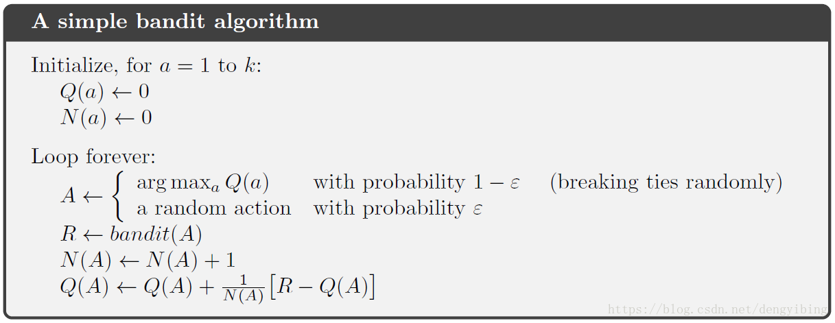
因为greedy 方法总是exploit，不会去explore，所以可以用 $\varepsilon \text{-greedy}$ 方法。

大多数时候（概率$1-\varepsilon$）正常greedy选择；只是偶尔（以概率$\varepsilon$）从所有actions中等概率的选择action，与action-value estimates独立

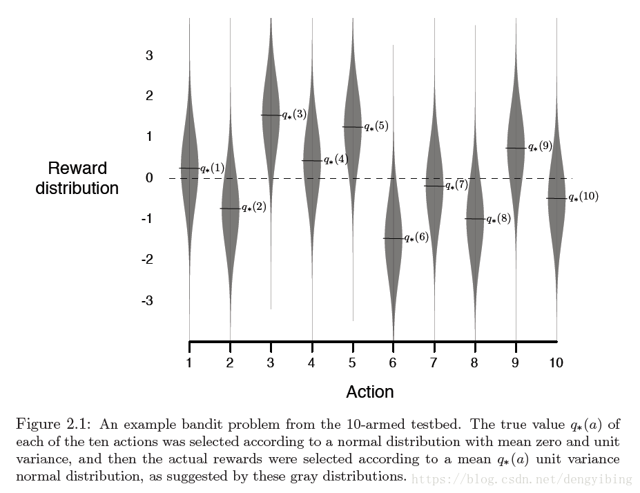
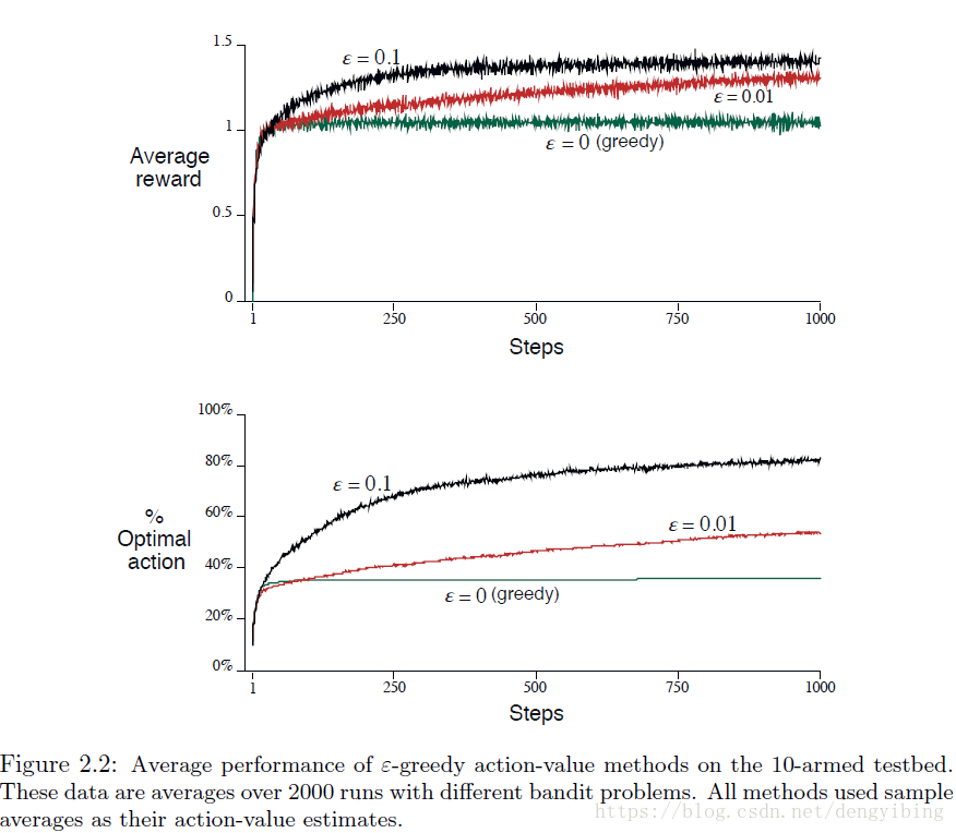
3. The 10-armed Testbed

用一个实例来说明 $\varepsilon \text{-greedy}$ 方法比 $\text{greedy}$ 方法要好

4. Incremental Implementation

我们迄今为止所讨论的action-value methods都将action-values估计为观察到的rewards的样本平均值。

考虑增量的计算这些averages，这样更高效，而且每一步的内存和计算都是固定的

$$Q_n \doteq \frac{R_1+R_2+ \cdots +R_{n-1}}{n-1}$$

$R_i$ now denote the reward received after the ith selection of this action

$Q_n$ denote the estimate of its action value after it has been selected n-1 times

则有

$$\begin{align*} Q_{n+1} & = \frac{1}{n}{\sum_{i=1}^{n}{R_i}} \\ & = \frac{1}{n}{(R_n+\sum_{i=1}^{n-1}{R_i})} \\ & = \frac{1}{n}{(R_n+(n-1)\frac{1}{n-1} \sum_{i=1}^{n-1}{R_i})} \\ & = \frac{1}{n}{(R_n+(n-1)Q_n)} \\ & = \frac{1}{n}{(R_n+nQ_n-Q_n)} \\ & = Q_n + \frac{1}{n} [R_n-Q_n] \end{align*}$$
对于n=1，有 $Q_2=R_1$

上述更新公式的一般形式将会一直出现在后面的文章中

$NewEstimate \leftarrow OldEstimate + StepSize\ [Target - OldEstimate]$

5. Tracking a Nonstationary Problem

averaging methods到目前为止对于stationary bandit problems是合适的，因为对bandit problems，reward probabilities不随时间变化

但是很多强化学习问题是nonstaionary的，在这种情况下，给最近的reward更大的权重更有意义。这种做法最流行的方法之一是使用恒定的step-size参数

这里average $Q_n$ 被修改为： $Q_{n+1} \doteq Q_n + \alpha [R_n - Q_n]$ ,其中 $\alpha \in (0,1]$ ，而且是常数。

This results in $Q_{n+1}$ being a weighted average of past rewards and the initial estimate $Q_1$:

$$\begin{align*} Q_{n+1} & = Q_n + \alpha [R_n - Q_n] \\ & =\alpha R_n + (1-\alpha)Q_n \\ & =\alpha R_n + (1-\alpha)[\alpha R_{n-1} + (1-\alpha)Q_{n-1}] \\ & =\alpha R_n + (1-\alpha)\alpha R_{n-1} + (1-\alpha)^2Q_{n-1} \\ & =\alpha R_n + (1-\alpha)\alpha R_{n-1} + (1-\alpha)^2R_{n-2} + \cdots+(1-\alpha)^{n-1}\alpha R_1 + (1-\alpha)^n Q_1 \\ & =(1-\alpha)^n Q_1 + \sum_{i=1}^n{\alpha(1-\alpha)^{n-i}R_i} \\ \end{align*}$$

有时，逐步改变步长参数是很方便的。但是不是所有的 $\alpha_n(a)$ 都保证收敛。

然而随机逼近理论中众所周知的结果为我们提供了确保以概率 1 收敛的条件：

$$\sum_{n-1}^{\infty}{\alpha_n(a)}=\infty \qquad \text{and} \qquad \sum_{n=1}^{\infty}{\alpha_n^2(a)}\lt\infty$$

6. Optimistic Initial Values

到目前为止，我们所讨论的所有方法在一定程度上取决于初始行动价值估计 $Q_1(a)$。用统计学的语言来说，这些方法偏向于他们的初步估计
但这并不普遍

7. Upper-Confidence-Bound(UCB) Action Selection

因为采用 $\varepsilon \text{-greedy}$ 方法，所以

根据其实际最佳的潜力，在非贪婪行为中进行选择会更好一些，同时考虑到它们的估计有多接近最大值以及这些估计值的不确定性

One effective way of doing this is to select actions according to:\
$A_t=\underset{\alpha}{arg\text{max}} [Q_t(a)+c\sqrt{\frac{\ln t}{N_t(a)}}]$

• $N_t(a)$ denotes the number of times that action a has been selected prior to time t
• the number c > 0 controls the degree of exploration

UCB常用在蒙特卡洛搜索树中

8. Gradient Bandit Algorithms

到目前为止，前面讲到的方法都是使用estimates来选择actions。这通常是一个好方法，但它不是唯一可能的方法。

这里考虑action a的numerical preference $H_t(a)$

相对preference才是要考虑的，这里根据soft-max distribution来考虑，根据更大的相对preference选择action

$$\Pr{(A_t=a)} \doteq \frac{e^{H_t(a)}}{\sum_{b=1}{k}{e^{H_t(a)}}} \doteq \pi_t(a)$$
这里的 $\pi_t(a)$ 就是后面常说的policy，在时刻t选择动作a的概率

学习算法为

$$\begin{align*} H_{t+1}(A_t) & \doteq H_t(A_t)+\alpha(R_t-\overline{R_t})(1-\pi_t(A_t)) & \text{, and} \\ H_{t+1}(A_t) & \doteq H_t(A_t)+\alpha(R_t-\overline{R_t})\pi_t(a) & \text{for all } a \neq A_t \end{align*}$$

这里 $\alpha \gt 0$ 是学习率

证明看书吧 Reinforcement Learning:An Introduction