戎易大数据 | 数据分析实操篇：关于2025 年全球产品库存数据集的探索（下）

最新推荐文章于 2025-11-23 18:54:45 发布

原创最新推荐文章于 2025-11-23 18:54:45 发布 · 572 阅读

5 ·

CC 4.0 BY-SA版权

文章标签：

#大数据 #数据分析 #数据挖掘 #人工智能 #AI编程 #chatgpt #python

深度学习拓展阅读同时被 2 个专栏收录

989 篇文章

订阅专栏

统计学

29 篇文章

订阅专栏

本文来源公众号“戎易大数据”，仅用于学术分享，侵权删，干货满满。

原文链接：https://mp.weixin.qq.com/s/VyQwShDWd8lO35CQ-cL2zA

https://blog.youkuaiyun.com/csdn_xmj/article/details/151566419

篇幅略长，后续内容请看上一篇！

产品间供应链关系探索

6.1 特征工程

# 特征工程：产品是否接近过期（假设存活时间小于1年为接近过期）data['Near_Expiry'] = np.where(data['life_cycle'] < 365, 1, 0)
# 特征工程：产品价格区间data['Price_Range'] = pd.cut(data['Price'], bins=[0, 100, 200, 300, 400, 500, np.inf],                             labels=['0-100', '100-200', '200-300', '300-400', '400-500', '500+'])
# 特征工程：库存状态（高、中、低）data['Stock_Status'] = pd.qcut(data['Stock Quantity'], q=3, labels=['Low', 'Medium', 'High'])
# 特征工程：产品类别编码category_mapping = {category: idx for idx, category in enumerate(data['Product Name'].unique())}data['Category_Code'] = data['Product Name'].map(category_mapping)

6.2 产品间关系分析

plt.figure(figsize=(25, 6))
plt.subplot(1, 3, 1)# 类别分布分析category_distribution = data['Product Name'].value_counts().reset_index()category_distribution.columns = ['Product Name', 'Count']sns.barplot(x='Product Name', y='Count', data=category_distribution, palette='spring')plt.title('商品分布', fontsize=16)plt.xlabel('商品名称', fontsize=12)plt.ylabel('数量', fontsize=12)for p in plt.gca().patches:    plt.gca().annotate(format(p.get_height(), '.0f'), (p.get_x() + p.get_width() / 2., p.get_height()), ha = 'center', va = 'center', xytext = (0, 5), textcoords = 'offset points')

# 类别间价格比较plt.subplot(1, 3, 2)sns.boxplot(x='Product Name', y='Price', data=data, palette='summer')plt.title('不同商品价格分布', fontsize=16)plt.xlabel('商品名称', fontsize=12)plt.ylabel('价格', fontsize=12)

# 类别间库存状态分析plt.subplot(1, 3, 3)sns.countplot(x='Product Name', hue='Stock_Status', data=data, palette='autumn')plt.title('不同商品库存状态分布', fontsize=16)plt.xlabel('商品名称', fontsize=12)plt.ylabel('数量', fontsize=12)for p in plt.gca().patches:    plt.gca().annotate(format(p.get_height(), '.0f'), (p.get_x() + p.get_width() / 2., p.get_height()), ha = 'center', va = 'center', xytext = (0, 5), textcoords = 'offset points')plt.show()

输出：

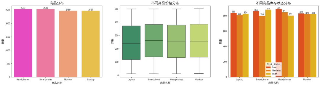
在低水平库存数量组别下，耳机以显著的库存优势位居首位。

中等水平库存数量组别中，耳机依然维持其领先地位。

高水平库存数量组别里，智能手机取代耳机成为排名第一的商品。

6.3 产品供应链时间维度分析

import matplotlib.dates as mdates
plt.figure(figsize=(20, 6))
# 制造日期分布plt.subplot(1, 3, 1)plt.hist(data['Manufacturing Date'], bins=30, edgecolor='black')plt.title('生产日期分布', fontsize=16)plt.xlabel('生产日期', fontsize=12)plt.ylabel('数量', fontsize=12)plt.gca().xaxis.set_major_formatter(mdates.DateFormatter('%Y-%m'))  # 设置日期显示格式
# 过期日期分布plt.subplot(1, 3, 2)plt.hist(data['Expiration Date'], bins=30, edgecolor='black')plt.title('过期日期分布', fontsize=16)plt.xlabel('过期日期', fontsize=12)plt.ylabel('数量', fontsize=12)plt.gca().xaxis.set_major_formatter(mdates.DateFormatter('%Y-%m'))  # 设置日期显示格式
# 有效期分布plt.subplot(1, 3, 3)sns.distplot(data['life_cycle'], bins=30, kde=True)plt.title('商品有效期分布', fontsize=16)plt.xlabel('有效期（天）', fontsize=12)plt.ylabel('数量', fontsize=12)
plt.tight_layout()plt.show()

输出：

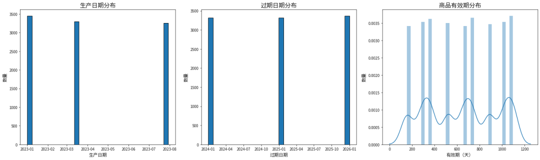
生产日期最早的是2023年1月，最晚的是2023年8月

过期日期最早的是2024年1月，最晚的是2026年1月

# 过期产品分析near_expiry_products = data[data['Near_Expiry'] == 1]print(f"Number of products near expiry: {len(near_expiry_products)}")print(near_expiry_products[['Product Name', 'Product Category', 'Expiration Date', 'life_cycle']])

输出：

Number of products near expiry: 2183     Product Name Product Category Expiration Date  life_cycle10        Monitor            Audio      2024-01-01         15511     Headphones            Audio      2024-01-01         29215     Smartphone           Mobile      2024-01-01         15522     Headphones            Audio      2024-01-01         15523         Laptop         Computer      2024-01-01         15525     Smartphone           Mobile      2024-01-01         15526        Monitor            Audio      2024-01-01         29228        Monitor            Audio      2024-01-01         29232     Smartphone           Mobile      2024-01-01         15533        Monitor            Audio      2024-01-01         15534         Laptop         Computer      2024-01-01         29237        Monitor            Audio      2024-01-01         15542         Laptop         Computer      2024-01-01         15544         Laptop         Computer      2024-01-01         29249     Headphones            Audio      2024-01-01         29257     Smartphone           Mobile      2024-01-01         15559     Smartphone           Mobile      2024-01-01         15565         Laptop         Computer      2024-01-01         29275     Headphones            Audio      2024-01-01         15576     Smartphone           Mobile      2024-01-01         29277         Laptop         Computer      2024-01-01         29279     Headphones            Audio      2024-01-01         15589        Monitor            Audio      2024-01-01         29295     Headphones            Audio      2024-01-01         155100    Headphones            Audio      2024-01-01         155101        Laptop         Computer      2024-01-01         292103    Smartphone           Mobile      2024-01-01         292104    Headphones            Audio      2024-01-01         292107    Smartphone           Mobile      2024-01-01         155110    Smartphone           Mobile      2024-01-01         155...           ...              ...             ...         ...9854   Smartphone           Mobile      2024-01-01         1559860   Smartphone           Mobile      2024-01-01         1559862      Monitor            Audio      2024-01-01         1559864      Monitor            Audio      2024-01-01         1559865      Monitor            Audio      2024-01-01         1559867   Headphones            Audio      2024-01-01         1559874      Monitor            Audio      2024-01-01         2929879   Smartphone           Mobile      2024-01-01         1559883       Laptop         Computer      2024-01-01         2929885   Headphones            Audio      2024-01-01         1559887   Smartphone           Mobile      2024-01-01         2929892   Smartphone           Mobile      2024-01-01         1559893   Smartphone           Mobile      2024-01-01         2929899      Monitor            Audio      2024-01-01         1559900   Headphones            Audio      2024-01-01         2929904      Monitor            Audio      2024-01-01         2929905   Smartphone           Mobile      2024-01-01         1559907       Laptop         Computer      2024-01-01         2929908      Monitor            Audio      2024-01-01         1559910      Monitor            Audio      2024-01-01         1559915   Smartphone           Mobile      2024-01-01         1559926   Headphones            Audio      2024-01-01         1559930       Laptop         Computer      2024-01-01         1559933   Smartphone           Mobile      2024-01-01         1559940   Smartphone           Mobile      2024-01-01         1559945      Monitor            Audio      2024-01-01         2929947       Laptop         Computer      2024-01-01         1559974       Laptop         Computer      2024-01-01         1559988   Headphones            Audio      2024-01-01         1559993   Smartphone           Mobile      2024-01-01         292
[2183 rows x 4 columns]

6.4 产品价格与库存关系分析

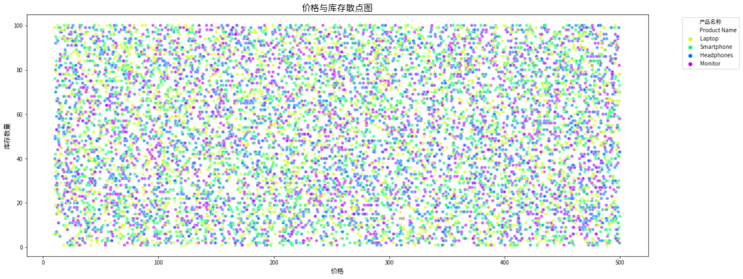
# 价格与库存散点图plt.figure(figsize=(20, 8))scatter_plot = sns.scatterplot(x='Price', y='Stock Quantity', hue='Product Name', data=data, alpha=0.6, palette='hsv')plt.title('价格与库存散点图', fontsize=16)plt.xlabel('价格', fontsize=12)plt.ylabel('库存数量', fontsize=12)plt.legend(bbox_to_anchor=(1.05, 1), loc='upper left', title='产品名称')plt.show()

输出：

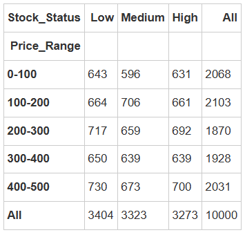
price_stock_table = pd.crosstab(data['Price_Range'], data['Stock_Status'], margins=True)price_stock_table

输出：

price_stock_table = price_stock_table.iloc[:-1]  # 去掉总计行price_stock_table.plot(kind='bar', stacked=True, figsize=(20, 6), cmap='tab10')plt.title('价格区间与库存状态交叉分析', fontsize=16)plt.xlabel('价格区间', fontsize=12)plt.ylabel('库存状态数量', fontsize=12)plt.xticks(rotation=0)plt.tight_layout()plt.show()

输出：

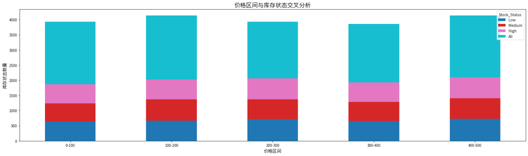
低库存状态

低库存状态下，商品总数为 3404 件，占总商品数（10000 件）的 34.04%。这表明有较大比例的商品处于库存紧张状态，需重点关注此类商品的供应链补货效率和市场需求响应速度。

价格区间分布差异：在价格区间 400 - 500 内，低库存商品数量最多，达 730 件。

中等库存状态

中等库存状态下，商品总数为 3323 件，占比 33.23%。这一库存水平的商品处于相对较为理想的状态，既能满足日常市场需求，又避免了过高库存带来的成本压力。

价格区间分布特征：价格区间 100 - 200 内中等库存商品数量最多，达 706 件。

高库存状态

高库存状态下，商品总数为 3273 件，占比 32.73%。这类商品占比较高，可能面临库存积压风险，增加了企业的仓储成本和资金占用压力，需要深入分析其滞销原因并制定针对性的促销或库存处理策略。

价格区间分布差异：价格区间 400 - 500 内高库存商品数量相对较多，达 700 件。

6.5 产品评分与供应链关系分析

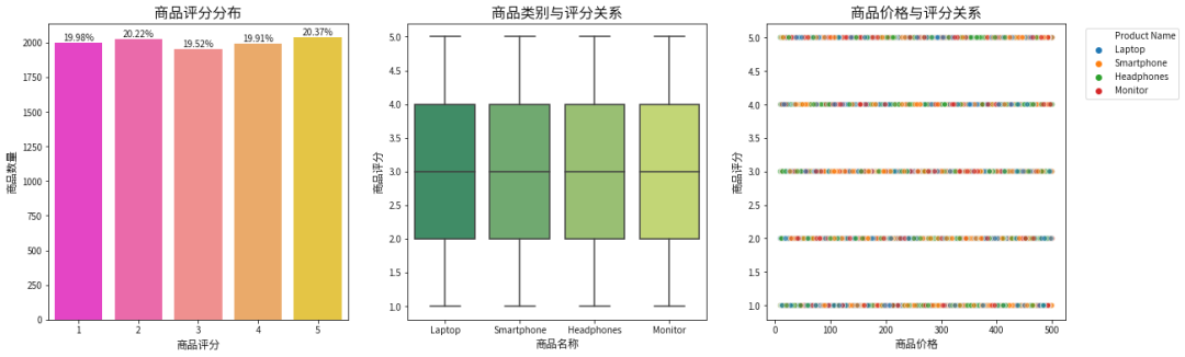
plt.figure(figsize=(20, 6))
# 产品评分分布plt.subplot(1, 3, 1)sns.countplot(x='Product Ratings', data=data,palette='spring')plt.title('商品评分分布', fontsize=16)plt.xlabel('商品评分', fontsize=12)plt.ylabel('商品数量', fontsize=12)for p in plt.gca().patches:    height = p.get_height()    plt.text(p.get_x() + p.get_width() / 2, height + 5, '{:1.2f}%'.format(height / len(data) * 100), ha='center', va='bottom')
# 评分与类别关系plt.subplot(1, 3, 2)sns.boxplot(x='Product Name', y='Product Ratings', data=data,palette='summer')plt.title('商品类别与评分关系', fontsize=16)plt.xlabel('商品名称', fontsize=12)plt.ylabel('商品评分', fontsize=12)
# 评分与价格关系plt.subplot(1, 3, 3)sns.scatterplot(x='Price', y='Product Ratings', hue='Product Name', data=data, alpha=0.6)plt.title('商品价格与评分关系', fontsize=16)plt.xlabel('商品价格', fontsize=12)plt.ylabel('商品评分', fontsize=12)plt.legend(bbox_to_anchor=(1.05, 1), loc='upper left')plt.show()

输出：

6.6 产品属性关联分析

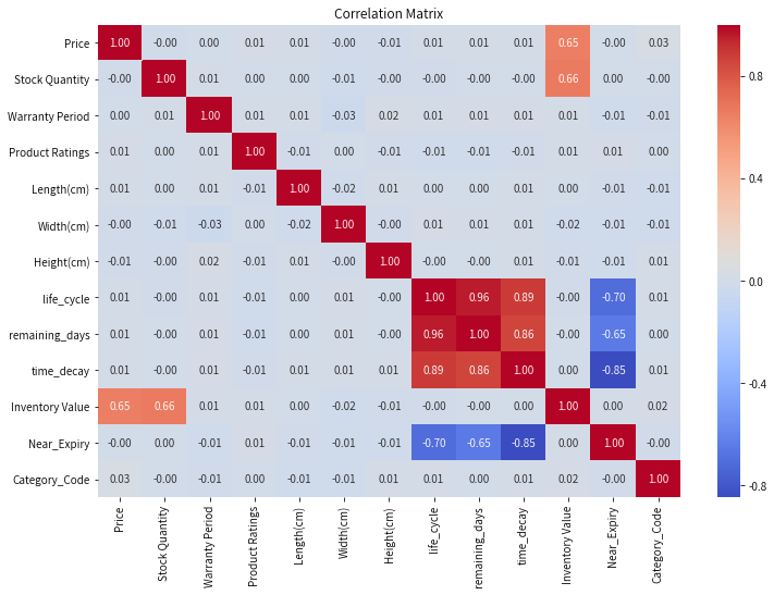
# 相关性矩阵features = data.select_dtypes(include=['int64', 'float64']).columnscorrelation_matrix = data[features].corr()plt.figure(figsize=(12, 8))sns.heatmap(correlation_matrix, annot=True, cmap='coolwarm', fmt='.2f')plt.title('Correlation Matrix')plt.show()

输出：

from mlxtend.preprocessing import TransactionEncoderfrom mlxtend.frequent_patterns import apriori, association_rules
# 创建事务数据集（示例：将产品属性组合成事务）product_attributes = data[['Product Name', 'Price_Range', 'Stock_Status', 'Near_Expiry']].copy()
# 将分类变量转换为哑变量product_attributes = pd.get_dummies(product_attributes, columns=['Product Name', 'Price_Range', 'Stock_Status'])
# 将数据转换为事务格式transactions = product_attributes.values.tolist()
# 应用Apriori算法te = TransactionEncoder()te_ary = te.fit(transactions).transform(transactions)df_transactions = pd.DataFrame(te_ary, columns=te.columns_)frequent_itemsets = apriori(df_transactions, min_support=0.01, use_colnames=True)
# 修复关联规则生成部分rules = association_rules(frequent_itemsets, metric='lift', min_threshold=1)
print(rules[['antecedents', 'consequents', 'support', 'confidence', 'lift']].head(20))

输出：

  antecedents consequents  support  confidence  lift0         (0)         (1)      1.0         1.0   1.01         (1)         (0)      1.0         1.0   1.0

结果表明,在这个数据集中，0 和 1 是完全相关的，每个事务同时包含这两个属性。这可能是因为数据中存在冗余或者重复的属性，或者是数据集结构过于简单，导致所有事务都包含相同的属性组合。

简易智能库存管理系统构建

from sklearn.linear_model import LinearRegressionimport datetime
# 数据层 - 加载产品数据class ProductDatabase:    def __init__(self, file_path):        self.data = pd.read_csv(file_path)
    def get_product_by_id(self, product_id):        return self.data[self.data['Product ID'] == product_id].iloc[0]
    def update_stock(self, product_id, new_stock):        self.data.loc[self.data['Product ID'] == product_id, 'Stock Quantity'] = new_stock
    def save_to_file(self, file_path):        self.data.to_csv(file_path, index=False)
# 业务逻辑层 - 库存管理class InventoryManager:    def __init__(self, product_db):        self.product_db = product_db
    def update_stock(self, product_id, quantity_change):        product = self.product_db.get_product_by_id(product_id)        new_stock = product['Stock Quantity'] + quantity_change        self.product_db.update_stock(product_id, new_stock)        return new_stock
    def predict_demand(self, product_id, days=30):        # 简单的线性回归预测示例        # 实际应用中需要更复杂的时间序列模型        product = self.product_db.get_product_by_id(product_id)        # 假设销售记录存储在另一个数据结构中        sales_data = pd.DataFrame({            'date': pd.date_range(end=datetime.datetime.now(), periods=30),            'sales': [product['Stock Quantity'] - i*2 for i in range(30)]  # 示例数据        })        sales_data['day'] = sales_data['date'].dt.dayofyear
        X = sales_data[['day']]        y = sales_data['sales']
        model = LinearRegression()        model.fit(X, y)
        future_days = pd.date_range(start=datetime.datetime.now(), periods=days)        future_df = pd.DataFrame({'day': future_days.dayofyear})        predictions = model.predict(future_df)
        return predictions
    def reorder_suggestion(self, product_id):        product = self.product_db.get_product_by_id(product_id)        # 简单的补货逻辑        if product['Stock Quantity'] < product['Stock Quantity'] * 0.2:            return f"Suggest reorder {product['Product Name']}, current stock: {product['Stock Quantity']}"        else:            return f"No reorder needed for {product['Product Name']}, current stock: {product['Stock Quantity']}"
# 应用层 - 用户界面class InventoryApp:    def __init__(self):        self.product_db = ProductDatabase('/home/mw/input/kucun8458/products.csv')        self.inventory_manager = InventoryManager(self.product_db)
    def run(self):        while True:            print("\nInventory Management System")            print("1. Update Stock")            print("2. Predict Demand")            print("3. Reorder Suggestion")            print("4. Exit")
            choice = input("Enter your choice: ")
            if choice == '1':                product_id = input("Enter Product ID: ")                quantity = int(input("Enter quantity change: "))                new_stock = self.inventory_manager.update_stock(product_id, quantity)                print(f"Updated stock to {new_stock}")
            elif choice == '2':                product_id = input("Enter Product ID: ")                days = int(input("Enter days to predict: "))                predictions = self.inventory_manager.predict_demand(product_id, days)                print(f"Predicted demand for next {days} days: {predictions}")
            elif choice == '3':                product_id = input("Enter Product ID: ")                suggestion = self.inventory_manager.reorder_suggestion(product_id)                print(suggestion)
            elif choice == '4':                self.product_db.save_to_file('/home/mw/input/kucun8458/products.csv')                print("Exiting...")                break
if __name__ == "__main__":    app = InventoryApp()    app.run()

输出：

Inventory Management System1. Update Stock2. Predict Demand3. Reorder Suggestion4. ExitUpdated stock to 303
Inventory Management System1. Update Stock2. Predict Demand3. Reorder Suggestion4. ExitPredicted demand for next 7 days: [245. 243. 241. 239. 237. 235. 233.]
Inventory Management System1. Update Stock2. Predict Demand3. Reorder Suggestion4. ExitExiting...