Day35

@浙大疏锦行

1. 三种不同的模型可视化方法：推荐torchinfo打印summary+权重分布可视化
2. 进度条功能：手动和自动写法，让打印结果更加美观
3. 推理的写法：评估模式

import torch
import torch.nn as nn
import torch.optim as optim
from sklearn.datasets import load_iris
from sklearn.model_selection import train_test_split
from sklearn.preprocessing import MinMaxScaler
import time
import matplotlib.pyplot as plt
 
# 设置GPU设备
device = torch.device("cuda:0" if torch.cuda.is_available() else "cpu")
print(f"使用设备: {device}")
 
# 加载鸢尾花数据集
iris = load_iris()
X = iris.data  # 特征数据
y = iris.target  # 标签数据
 
# 划分训练集和测试集
X_train, X_test, y_train, y_test = train_test_split(X, y, test_size=0.2, random_state=42)
 
# 归一化数据
scaler = MinMaxScaler()
X_train = scaler.fit_transform(X_train)
X_test = scaler.transform(X_test)
 
# 将数据转换为PyTorch张量并移至GPU
X_train = torch.FloatTensor(X_train).to(device)
y_train = torch.LongTensor(y_train).to(device)
X_test = torch.FloatTensor(X_test).to(device)
y_test = torch.LongTensor(y_test).to(device)
 
class MLP(nn.Module):
    def __init__(self):
        super(MLP, self).__init__()
        self.fc1 = nn.Linear(4, 10)  # 输入层到隐藏层
        self.relu = nn.ReLU()
        self.fc2 = nn.Linear(10, 3)  # 隐藏层到输出层
 
    def forward(self, x):
        out = self.fc1(x)
        out = self.relu(out)
        out = self.fc2(out)
        return out
 
# 实例化模型并移至GPU
model = MLP().to(device)
 
# 分类问题使用交叉熵损失函数
criterion = nn.CrossEntropyLoss()
 
# 使用随机梯度下降优化器
optimizer = optim.SGD(model.parameters(), lr=0.01)
 
# 训练模型
num_epochs = 20000  # 训练的轮数
 
# 用于存储每100个epoch的损失值和对应的epoch数
losses = []
 
start_time = time.time()  # 记录开始时间
 
for epoch in range(num_epochs):
    # 前向传播
    outputs = model(X_train)  # 隐式调用forward函数
    loss = criterion(outputs, y_train)
 
    # 反向传播和优化
    optimizer.zero_grad() #梯度清零，因为PyTorch会累积梯度，所以每次迭代需要清零，梯度累计是那种小的bitchsize模拟大的bitchsize
    loss.backward() #  反向传播计算梯度
    optimizer.step() # 更新参数
 
    # 记录损失值
    if (epoch + 1) % 200 == 0:
        losses.append(loss.item()) # item()方法返回一个Python数值，loss是一个标量张量
        print(f'Epoch [{epoch+1}/{num_epochs}], Loss: {loss.item():.4f}')
    
    # 打印训练信息
    if (epoch + 1) % 100 == 0: # range是从0开始，所以epoch+1是从当前epoch开始，每100个epoch打印一次
        print(f'Epoch [{epoch+1}/{num_epochs}], Loss: {loss.item():.4f}')
 
time_all = time.time() - start_time  # 计算训练时间
print(f'Training time: {time_all:.2f} seconds')
 
 
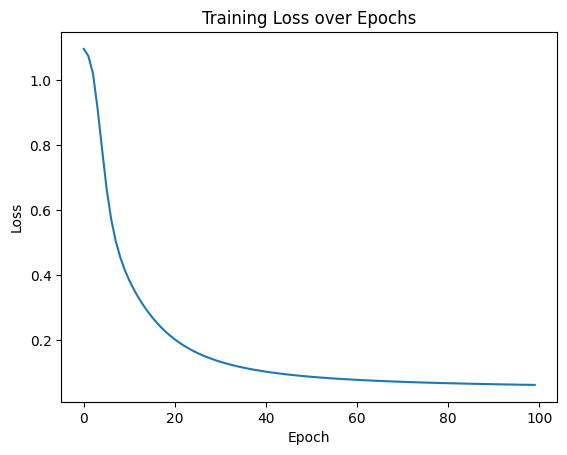
# 可视化损失曲线
plt.plot(range(len(losses)), losses)
plt.xlabel('Epoch')
plt.ylabel('Loss')
plt.title('Training Loss over Epochs')
plt.show()

#  nn.Module 的内置功能，直接输出模型结构
print(model)
 
 
MLP(
  (fc1): Linear(in_features=4, out_features=10, bias=True)
  (relu): ReLU()
  (fc2): Linear(in_features=10, out_features=3, bias=True)
)
 
 
# nn.Module 的内置功能，返回模型的可训练参数迭代器
for name, param in model.named_parameters():
    print(f"Parameter name: {name}, Shape: {param.shape}")
 
 
Parameter name: fc1.weight, Shape: torch.Size([10, 4])
Parameter name: fc1.bias, Shape: torch.Size([10])
Parameter name: fc2.weight, Shape: torch.Size([3, 10])
Parameter name: fc2.bias, Shape: torch.Size([3])