


提示:文章写完后,目录可以自动生成,如何生成可参考右边的帮助文档
目录
前言
本文章利用简单的MLP对加州房价进行预处理和预测
课程是李沐大神的动手学深度学习(pytorch)
竞赛地址:California House Prices | Kaggle
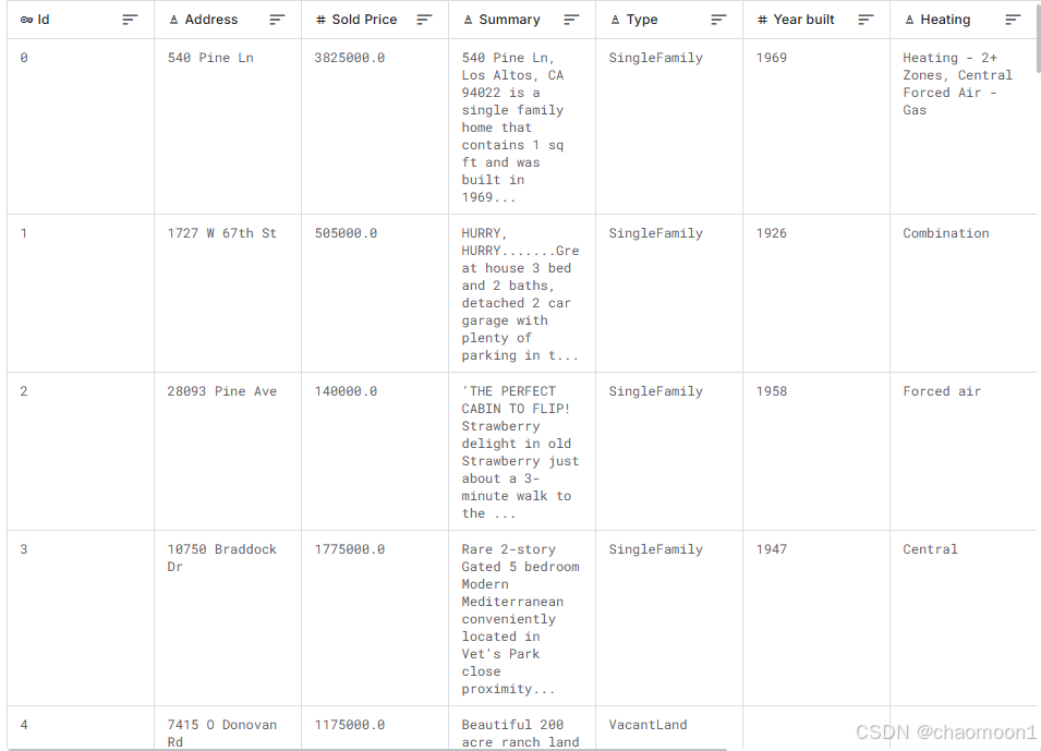
一、认识数据
House Prices数据集分为train(即训练)数据和test(即测试)数据,其中,训练集含有47325个样本,40个属性(包括序号),一个标签(Sold Price,即房价);测试集含有31559个样本,40个属性。
需要做的工作:根据测试集的属性预测每个样本的房价。
二、数据预处理
2.1定性分析
ID:每个房子特有的号码
Address:房子地址
Sold Price:房子实际出售的价格,在测试集中是需要预测的部分
Summary:房子信息的摘要
Type:房子类型
Year Built:房子建造年份
Heating:供暖设施
Cooling:供冷设施
Parking:停车区域
Lot:占用土地
Bedrooms:卧室数
Bathrooms:浴室数
Full Bathrooms:完整的浴室数
Total interior livable area:总内部可居住面积
Total spaces:总空间
Garage spaces:车库空间
Region:行政区
Elementary School、score、distance:小学名称,分数和距离
Middle School、score、distance:初中名称,分数和距离
High School、score、distance:高中名称,分数和距离
Flooring:地板
Heating features:加热功能
Cooling features:降热功能
Appliances included:包含的设备
Laundry features:洗衣功能
Parking features:停车功能
Tax assessed value:税财产评估
Annual tax amount:年纳税额
Listed On:列入名单的日期
Listed Price:标明价格(不是最终买的价格,房子还需要拍卖起价)
Last Sold On:上次出售的日期
Last Sold Price:上次出售的价格
City:城市
Zip:邮编
State:所在州
2.2缺失值处理
2.2.1缺失值统计
训练集数据缺失情况, 和它们对应的意义为:
import pandas as pd

# 读取数据
train_data = pd.read_csv('F:/data/california-house-prices/train.csv')

total = train_data.isnull().sum().sort_values(ascending=False)
percent =(train_data.isnull().sum()/train_data.isnull().count()).sort_values(ascending=False)
missing_data = pd.concat([total, percent], axis=1, keys=['Total', 'Percent'])
print(missing_data.head(20))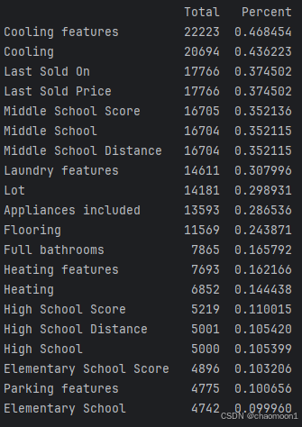
2.2.2 填充缺失值
缺失数据的变量有很多,处理情况可以分为如下几类:
(1)缺失多
直接数据集中剔除哪些存在大量缺失值的变量 缺失量比较多的Cooling Feature、Cooling是由于房子没有降温设施。 由于缺失量比较多,缺失率超过40%,我们直接移除这几个变量。
train_data.drop(missing_data[missing_data['Percent'] > .4].index, axis=1, inplace=True)(2)卧室数属性
卧室列包含数字和文字描述,现将文字改为数字
再填充空缺值为2(众数为2)
# 处理 Bedrooms 列,计算数量
def convert_bedrooms(bedrooms):
  # 尝试转换为数字
  try:
  # 如果是纯数字字符串,返回它的浮点数形式
     return float(bedrooms)
  except ValueError:
     # 如果不是数字字符串,尝试分割字符串并计算总和
     values = bedrooms.split(',')  # 用,分开
     return len(values)
# 应用转换函数
all_features['Bedrooms'] = all_features['Bedrooms'].apply(convert_bedrooms)
all_features['Bedrooms'] = all_features['Bedrooms'].fillna(2.0)
(3)浴室数属性
浴室有Bathroom和Full Bathrooms两列,空缺值先互相填充,再用众数填充
all_features['Bathrooms'] = all_features['Bathrooms'].fillna(all_features['Full bathrooms'])
all_features['Bathrooms'] = all_features['Bathrooms'].fillna(2.0)

all_features['Full bathrooms'] = all_features['Full bathrooms'].fillna(all_features['Bathrooms'])
all_features['Full bathrooms'] = all_features['Full bathrooms'].fillna(all_features['Full bathrooms'].mode())
(4)其他属性
其他都用众数或平均数填充
例:
all_features['Elementary School Score'] = all_features['Elementary School Score'].fillna(all_features['Elementary School Score'].mode().values[0])
all_features['High School Score'] = all_features['High School Score'].fillna(all_features['High School Score'].mode())
all_features['Tax assessed value'] = all_features['Tax assessed value'].fillna(all_features['Listed Price'] * 0.66)
三、特征分析
3.1 房价分析
首先对房价进行分析,画出房价的分布图为:
from matplotlib import pyplot as plt

train_data = pd.read_csv('dataset/california-house-prices/train.csv')
sold_price = train_data['Sold Price']
plt.hist(sold_price, bins=1000)
plt.xlim(0,10000000)
plt.xlabel('Sold Price')
plt.ylabel('Frequency')
plt.title('Distribution of Sold Price')
plt.show()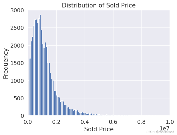
3.2 房价属性的关系
在此先分析房价与属性的关系,其中数值型的属性有
import numpy as np


numeric_cols = train_data.select_dtypes(include=np.number).columns
print(numeric_cols)


Index(['Id', 'Sold Price', 'Year built', 'Total interior livable area',
       'Total spaces', 'Garage spaces', 'Elementary School Score',
       'Elementary School Distance', 'High School Score',
       'High School Distance', 'Tax assessed value', 'Annual tax amount',
       'Listed Price', 'Zip'],
      dtype='object')
相关性分析:(颜色越浅,对应的像个特征的相关性越大)
import seaborn as sns
corrmat = train_data[numeric_cols].corr()
f, ax = plt.subplots(figsize=(12, 9))
sns.heatmap(corrmat, vmax=.8, square=True)
plt.show()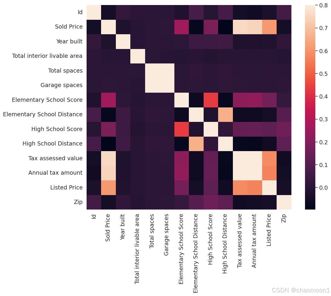
取相关性最大的10个进一步分析:
k = 10
cols = corrmat.nlargest(k, 'Sold Price')['Sold Price'].index
cm = np.corrcoef(train_data[cols].values.T)
sns.set(font_scale=1.25)
hm = sns.heatmap(cm, cbar=True, annot=True, square=True, fmt='.2f', annot_kws={'size': 10}, yticklabels=cols.values, xticklabels=cols.values)
plt.xticks(rotation = 90)
plt.show()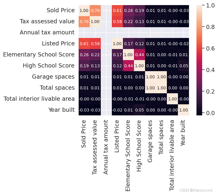
可以看到,像Listed Price,Annual Tax amount等与Sold Price有很强的正相关性,但是Tax assessed value和Annual Tax amount之间也有很强的正相关性,大概是0.66倍,那这两列只取一列就行。
进一步采用皮尔逊相关分析法对所有属性和房价进行分析:
def spearman(df,cols):
  spr = pd.DataFrame()
  spr['feature'] = cols
  spr['corr'] = [df[f].corr(df['Sold Price'], 'spearman') for f in cols]
  spr = spr.sort_values('corr')
  plt.figure(figsize=(6, 0.25*len(cols)))
  sns.barplot(data=spr, y='feature', x='corr', orient='h')

spearman(train_data,numeric_cols)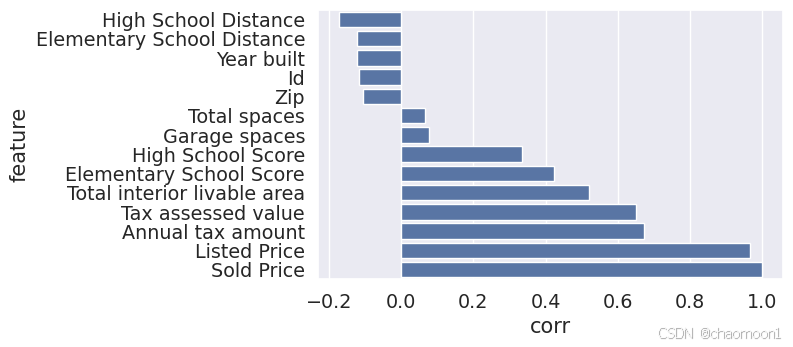
以上是对数值型的数据分析,下面对字符型的数据进行分析
obj_cols = train_data.select_dtypes(exclude=np.number).columns
obj_cols = obj_cols.drop(['Address','Summary','Elementary School','Middle School','High School','State'])
print(obj_cols)

Index(['Type', 'Heating', 'Cooling', 'Parking', 'Bedrooms', 'Region',
       'Flooring', 'Heating features', 'Cooling features',
       'Appliances included', 'Laundry features', 'Parking features',
       'Listed On', 'Last Sold On', 'City'],
      dtype='object')
为了使得特征分析顺利进行,首先对字符串型的属性转换到数值型。
转换的规则是:对于字符型属性,按照各个类型的属性的不同取值时房价的均值排高低,按此顺序从低往高,给属性的不同取值赋予1,2,3,4……,使得其变成数值型。
def trans_num(df,feat):
  ordering = pd.DataFrame()
  ordering['feat'] = df[feat].unique()
  ordering.index = ordering.feat
  ordering['spmean'] = df[[feat,'Sold Price']].groupby(feat).mean()['Sold Price']
  ordering = ordering.sort_values('spmean')
  ordering['ordering'] = range(1, ordering.shape[0]+1)
  ordering = ordering['ordering'].to_dict()
  for cat, o in ordering.items():
    df.loc[df[feat]==cat, feat+'_T'] = o
num_transformed = []
for q in obj_cols:
  num_transformed.append(q+'_T')
  trans_num(train_data,q)
经过转换后的属性全部为数值型,这时有利于进行分析。
同样采用皮尔逊相关分析法对所有属性和房价进行分析。
spearman(train_data,num_transformed)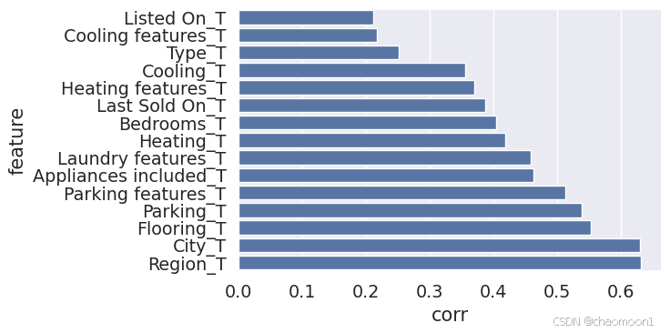
根据以上讨论,去掉部分互相相关性强的属性,选择作为房价分析的特征有:
'Bathrooms','Full bathrooms','Elementary School Score','High School Score','Listed Price','Tax assessed value','Type','Listed On','Bedrooms','Heating','Parking','City','Region','Cooling','Appliances included'
四、回归前的准备
4.1 预处理
此前是对训练集预处理,现在加上测试集,再进行独热编码,标准化等操作
import pandas as pd
import torch
import torch.nn as nn
import torch.optim as optim
from torch.utils.data import DataLoader
from sklearn.preprocessing import StandardScaler

# 设置设备
device = torch.device("cuda" if torch.cuda.is_available() else "cpu")

# 读取数据
train_data = pd.read_csv('dataset/california-house-prices/train.csv')
test_data = pd.read_csv('dataset/california-house-prices/test.csv')

batch_size = 1024
# 数据预处理
all_features = pd.concat((train_data.iloc[:,4:],test_data.iloc[:,4:]))
all_features = all_features[['Bathrooms','Full bathrooms','Elementary School Score','High School Score','Listed Price','Tax assessed value','Type','Listed On','Bedrooms','Heating','Parking','City','Region','Cooling','Appliances included']]

# 处理 Bedrooms 列,计算数量
def convert_bedrooms(bedrooms):
  # 尝试转换为数字
  try:
  # 如果是纯数字字符串,返回它的浮点数形式
     return float(bedrooms)
  except ValueError:
     # 如果不是数字字符串,尝试分割字符串并计算总和
     values = bedrooms.split(',')  # 用,分开
     return len(values)
# 应用转换函数
all_features['Bedrooms'] = all_features['Bedrooms'].apply(convert_bedrooms)
all_features['Bedrooms'] = all_features['Bedrooms'].fillna(2.0)

all_features['Bathrooms'] = all_features['Bathrooms'].fillna(all_features['Full bathrooms'])
all_features['Bathrooms'] = all_features['Bathrooms'].fillna(all_features['Bathrooms'].mode().values[0])

all_features['Full bathrooms'] = all_features['Full bathrooms'].fillna(all_features['Bathrooms'])
all_features['Full bathrooms'] = all_features['Full bathrooms'].fillna(all_features['Full bathrooms'].mode().values[0])

all_features['Elementary School Score'] = all_features['Elementary School Score'].fillna(all_features['Elementary School Score'].mode().values[0])
all_features['High School Score'] = all_features['High School Score'].fillna(all_features['High School Score'].mode().values[0])
all_features['Type'] = all_features['Type'].fillna(all_features['Type'].mode().values[0])
all_features['Region'] = all_features['Region'].fillna(all_features['Region'].mode().values[0])
all_features['Tax assessed value'] = all_features['Tax assessed value'].fillna(all_features['Listed Price'] * 0.66)


def convert_parkings(parkings):
   if parkings == '0 spaces' :
       return 0
   elif isinstance(parkings, float):
       return parkings
   else:
      return 1

all_features['Parking'] = all_features['Parking'].apply(convert_parkings)

def convert_heating(heating):
   if heating == 'None' :
       return 1
   elif isinstance(heating, float):
       return heating
   else:
      values = heating.split(',')
      return len(values)

def convert_appliance(appliances):
  if isinstance(appliances, float):
       return appliances
  else:
    values = appliances.split(',')
    return len(values)


all_features['Heating'] = all_features['Heating'].apply(convert_heating)

all_features['Appliances included'] = all_features['Appliances included'].apply(convert_appliance)
all_features['Appliances included'] = all_features['Appliances included'].fillna(all_features['Appliances included'].mode().values[0])

all_features['Cooling'] = all_features['Cooling'].fillna(all_features['Cooling'].mode().values[0])


# 新特征提取
all_features['Listed On'] = 2023  - pd.to_datetime(all_features['Listed On']).dt.year


# 独热编码
all_features = pd.get_dummies(all_features, dummy_na=True)
all_features = all_features.fillna(0)
all_features = all_features.astype('float32')


# 标准化
scaler = StandardScaler()
numeric_features = all_features.select_dtypes(include=['float32', 'int']).columns
all_features[numeric_features] = scaler.fit_transform(all_features[numeric_features])
all_features[numeric_features] = all_features[numeric_features].fillna(0)


# 划分训练集和测试集
n_train = train_data.shape[0]
train_features = torch.tensor(all_features[:n_train].values, dtype=torch.float32).to(device)
train_labels = torch.tensor(train_data['Sold Price'].values.reshape(-1, 1), dtype=torch.float32).to(device)
train_dataset = torch.utils.data.TensorDataset(train_features, train_labels)
test_features = torch.tensor(all_features[n_train:].values, dtype=torch.float32).to(device)


# 定义数据加载器
train_loader = DataLoader(dataset=train_dataset, batch_size=batch_size, shuffle=True)
五、回归
现在训练集的选取的属性和标签准备就位,测试集的选取的属性也预处理完毕,可以进行测试集的回归预测了。
我只是用了纯MLP进行回归,损失函数用SmoothL1Loss更平滑,优化器用Adam,对学习率不太敏感,正则用weight_decay,没有是丢弃法,其实效果一样,为了防止过拟合还用了k折交叉验证。
input_size = train_features.shape[1]
# 定义模型
class Net(nn.Module):
    def __init__(self):
        super(Net, self).__init__()
        self.layers = nn.Sequential(
            nn.Linear(input_size, 2048),
            nn.ReLU(),
            nn.Linear(2048, 1024),
            nn.ReLU(),
            nn.Linear(1024, 512),
            nn.ReLU(),
            nn.Linear(512, 256),
            nn.ReLU(),
            nn.Linear(256, 128),
            nn.ReLU(),
            nn.Linear(128, 64),
            nn.ReLU(),
            nn.Linear(64, 1),
            nn.ReLU()
        )
        self.apply(self.init_weights)

    def init_weights(self, m):
        if isinstance(m, nn.Linear):
            nn.init.xavier_uniform_(m.weight)

    def forward(self, x):
        return self.layers(x)

model = Net().to(device)
# 定义损失函数
loss = torch.nn.SmoothL1Loss()
# 定义优化器
optimizer = optim.Adam(model.parameters(), lr=0.001, weight_decay=1e-4)
infeatures = train_features.shape[1]

# 计算相对误差
def log_rmse(net, features, labels):
    clipped_preds = torch.clamp(net(features), 1,float('inf'))
    rmse = torch.sqrt(loss(torch.log(clipped_preds),torch.log(labels)))
    return rmse.item()

#训练
def train(num_epochs, train_features, train_labels, test_features, test_labels,device):
    train_ls, test_ls = [], []
    for epoch in range(num_epochs):
        for batch_idx, data in enumerate(train_loader,0):
            inputs, target = data
            inputs, target = inputs.to(device), target.to(device)
            optimizer.zero_grad()
            l = loss(model(inputs), target)
            l.backward()
            optimizer.step()


        train_ls.append(log_rmse(model, train_features, train_labels))
        if test_labels is not None:
            test_ls.append(log_rmse(model, test_features, test_labels))
            print(f'Epoch {epoch + 1}, train log rmse {train_ls[-1]:.4f}, test log rmse {test_ls[-1]:.4f}')
        else:
            print(f'Epoch {epoch + 1}, train log rmse {train_ls[-1]:.4f}')
    return train_ls, test_ls

# K折交叉验证
def get_k_fold_data(k, i, X, y):
    assert k > 1
    fold_size = X.shape[0] // k
    X_train, y_train = None, None
    for j in range(k):
        idx = slice(j * fold_size, (j + 1) * fold_size)
        X_part, y_part = X[idx, :], y[idx]
        if j == i:
            X_valid, y_valid = X_part, y_part
        elif X_train is None:
            X_train, y_train = X_part, y_part
        else:
            X_train = torch.cat((X_train, X_part), dim=0)
            y_train = torch.cat((y_train, y_part), dim=0)
    return X_train, y_train, X_valid, y_valid

# 返回训练和验证误差的平均值
def k_fold(k, X_train, y_train, num_epochs):
    train_l_sum, valid_l_sum = 0, 0
    for i in range(k):
        data = get_k_fold_data(k, i, X_train, y_train)
        train_l, valid_l = train(num_epochs, *data, device=device)
        train_l_sum += train_l[-1]
        valid_l_sum += valid_l[-1]
        print(f'fold {i + 1}, train log rmse {train_l[-1]:.4f}, valid log rmse {valid_l[-1]:.4f}')
    return train_l_sum / k, valid_l_sum / k

k,num_epochs = 5, 1000
train_l, valid_l = k_fold(k, train_features, train_labels, num_epochs)
print(f'{k}-fold validation: avg train log rmse {train_l:.4f}, avg valid log rmse {valid_l:.4f}')

# 预测
def predict(model, features):
    model.eval()
    with torch.no_grad():
        features = features.to(device)
        preds = model(features).detach().cpu().numpy()
    return preds
# 保存预测结果
preds = predict(model, test_features)
test_data['Sold Price'] = preds
test_data[['Id', 'Sold Price']].to_csv('dataset/california-house-prices/CA-house-price-submission.csv', index=False)
六、提交结果

MLP的效果没那么好,可能是在数据预处理的部分还没有做好,在特征工程仍需要下功夫,可以用automl来自动提取特征,也可以用集成模型或决策树等其他机器学习方法,分数在0.13附近,本人学术尚浅,暂未掌握。
总结
利用MLP对加州房价的预测
var code = "d4928ff5-2216-4e92-b1eb-c8a4c4d1244a"


 934
934

 被折叠的 条评论
为什么被折叠?
被折叠的 条评论
为什么被折叠?
 到【灌水乐园】发言


