新手实战详解：Kaggle房价预测 + 课程竞赛：加州2020年房价预测（动手学深度学习v2）

---

本文仅作为个人学习笔记用，如有错误请指正，欢迎大家讨论学习。本博客内容来自动手学深度学习

---

项目场景：

作为在B站“不那么认真”的学习到这节课的小白，当学到这节课以为能来一次帅气的实战时，结果自然是被拷打了；项目使用的方法与老师在课上的框架基本一致，进行分数优化时也作出了相应更改，所以主要以李沐老师的项目为思路。

项目来自李沐老师在kaggle上举行的竞赛，虽然是几年前的竞赛但是作为新手第一次尝试也未尝不可（相关链接放在文章末）

任务是根据房屋信息预测房屋销售价格，例如卧室、生活区域、位置、附近的学校和卖家摘要。该数据包括 2020 年在加利福尼亚州售出的房屋，测试数据集中的房屋售出率晚于训练数据集中的房屋售出。此外，私人排行榜上的房屋在公共排行榜上的房屋之后被出售（假如训练集是前三个月，测试集就是后三个月，那么公共排行榜的数据来自测试集的后三个月，私人排行榜为再后三个月）。

---

数据集的思考

很重要

之前的实战经验基本为0，一个是毕设的葡萄叶叶部病害识别和李沐老师实战课上的一个小项目以外没有过多接触了。
但是本次实战的数据集复杂度提高，给出的训练集标签总计就有41列，导致的问题是简单的数据集清洗后，想直接进行独热编码时，内存直接爆了（70多GB啊）。给我带来了沉重地思考，老师明明在课上是这么写的啊，怎么换一个数据集就不得劲了呢。

数据选择

没错当我看了标签内的详细数据沉默了，一些文字数据的比例确实不太对劲，比如这种：

两万多个不同的数据，想做成独热编码，咱这小电脑属实扛不住啊，所以虽然深度学习是黑盒但我们面对数据集可不能这样（所以沐神十行的代码含金量还在提升）。那么，面对一些难以处理的数据集，我的方法显然是选择Drop了。

随机森林（Random Forest）

当然，这明显是新手听到的最多且最容易的方法；虽然只是新手实战，但是我在想这么随意的丢弃标签数据真的好吗，于是经过一番搜索，发现了随机森林（Random Forest） 方法，它显示的特征重要性表示每个特征对模型预测结果的贡献程度。于是我赶紧在数据集上运行了该测试。这么一看，发现很多文字的重要性并没有那么高（可以心安理得的drop了）。经过一番筛选我将以下标签drop了

'Address', 'Summary', 'State', 'Heating', 'Cooling', 'Elementary School','Middle School', 
'High School', 'Flooring', 'Cooling features', 'Parking features', 'Appliances included', 
'Laundry features', 'Laundry features', 'Last Sold On', 'Listed On'

稀疏类别合并

当然，我同时也学习到了一些数据筛选的方法，比如对于一些有用的文字数据集，明明有的数据占比尚可，但是被一些other数据拖累了就要drop属实可惜,比如Type类型，我就很想保留前两个比例高的内容，那么就可以采用稀疏类别合并的方法，将other里面的内容占比不足x%（x自定义，本文采用1%）的内容归为other，这样大概率就只会有SingleFamily、Condo、Other三种数据，这样就将原本Other类里面的8021个数据直接变成了other这个单一数据。

comb_columns = ['Type', 'Region', 'Heating features', 'City']#需要合并的标签

特殊的数据标签

在我搜集各路门派的“武林秘籍”时，发现一位佬的想法挺有意思的，那就是对BedRoom这种数字文字混合的内容进行处理。原文链接https://www.kaggle.com/competitions/california-house-prices/discussion/254451

文本内容描述的是拥有的若干卧室，并用,隔开，于是可以将文本的逗号数+1，得到卧室的数量

要统计逗号的数量，可以使用collections包里的Counter类，由于列表中的部分数字使用字符串形式存放的，在此之前判断一下内容是否为数字

数据集处理代码

之前的随机森林就不贴上来了，因为主要是想用一用，理解也不透彻，可以看看其他佬的相关贴

import hashlib
import os
import tarfile
import zipfile
import requests
import numpy as np
import pandas as pd
import torch
from torch import nn
from d2l import torch as d2l
import unicodedata
from collections import Counter

#加载数据集
train_data = pd.read_csv('./01_data/02_DataSet_Kaggle_House/california-house-prices/train.csv')
test_data = pd.read_csv('./01_data/02_DataSet_Kaggle_House/california-house-prices/test.csv')
print(train_data.shape)

#选择Drop标签
irrelevant_columns = ['Address', 'Summary', 'State', 'Heating', 'Cooling', 'Elementary School',
                      'Middle School', 'High School', 'Flooring', 'Cooling features', 'Parking features',
                      'Appliances included', 'Laundry features', 'Laundry features', 'Last Sold On', 'Listed On']
                      
#选择并稀疏类别标签
comb_columns = ['Type', 'Region', 'Heating features', 'City']

#特殊的数据标签
List1 = ['Bedrooms','Parking']

####
这里按照课程项目思路，先去掉训练集售卖价格的标签（因为测试集并没有这个标签），再删掉
irrelevant_columns内的标签
###
train_features1 = train_data.drop(columns=['Sold Price'])
train_features1 = train_features1.drop(columns=irrelevant_columns)
test_features1 = test_data.drop(columns=irrelevant_columns)

#拼接两个数据集，这里就会让Id标签消失
all_features = pd.concat((train_features1.iloc[:,1:],test_features1.iloc[:,1:]))


#List1处理（特殊标签处理）
def count_comma(s):
    dic = Counter(s)
    return dic[',']

def is_number(s):
    try:
        float(s)
        return True
    except ValueError:
        pass

    try:
        unicodedata.numeric(s)
        return True
    except (TypeError, ValueError):
        pass

    return False

def comma_to_number(features,list):
    # 先拷贝，用于去除pd拷贝错误
    X = features.reset_index(drop=True).copy()
    for cols in list:
        for i,item in enumerate(X[cols]):
            if not is_number(item):
                X.loc[i,cols] = count_comma(item)+1
        X[cols] = X[cols].astype('float')
    return X

all_features = comma_to_number(all_features,List1)#到这里List内的标签就被我们数字化处理了

# 自动合并稀疏类别函数（基于指定列）
def combine_rare_categories(df, columns, threshold=1):
    for col in columns:
        if col in df.columns:  # 确保列在数据集中
            value_counts = df[col].value_counts(normalize=True) * 100
            rare_categories = value_counts[value_counts < threshold].index  # 选择占比低于阈值的稀疏类别
            df[col] = df[col].apply(lambda x: 'Other' if x in rare_categories else x)  # 合并稀疏类别为 'Other'
    return df
#合并稀疏向
df_combined = combine_rare_categories(all_features, comb_columns, threshold=1)

# 查看合并后的数据集
print(df_combined.head())

#自此我们保存的all_features进行了drop不需要的项，以及合并稀疏矩阵，对bedroom和parking进行了数字化处理
all_features.to_csv('all_features.csv', index=False)
#当时数据处理每一步都会进行很久，而且思路不是很明朗所以我们把辛辛苦苦处理的all_features
#采用csv格式保存下来，便于后续直接使用

开始炼丹：

之后可以按照李沐老师课上教的项目的方法愉快的玩耍了，具体方法也许过两天就更了（今晚更）

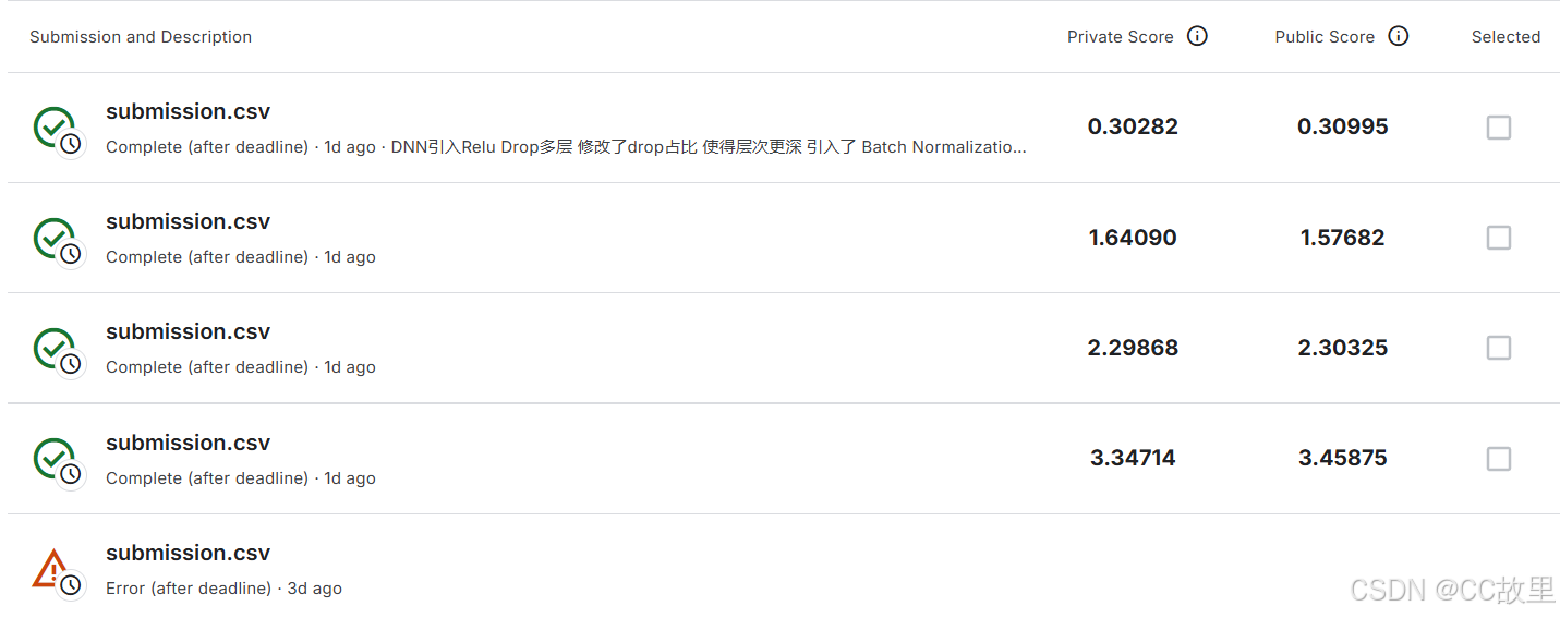
由于我已经将all_features保存为csv文件了，为了代码不那么拥挤我重新创建了一个py文件并且在jupyter上运行，和pycharm上不会有区别，只不过可以灵活执行代码块了。第一版的分数是在3.3左右，代码和老师给的完全一致，除了最后保存的submission文件中，老师的标签和竞赛的标签不一致，需修改。
submission = pd.concat([test_data['Id'],test_data['SalePrice']],axis=1)我们要将SalePrice改为Sold Price这样在kaggle上就可以正确提交我们的submission文件了。

第二版时主要修改了网络结构，感觉单层结构面对复杂的数据集难免会比较吃力，并且引入了梯度裁剪，然后调参得到了2.2~1.6的分数

第三版时引入了更多的方法来提高模型泛化能力，比如自动调整学习率，在网络层上 引入了 Batch Normalization详细代码如下

import hashlib
import os
import tarfile
import zipfile
from sched import scheduler

import requests
import numpy as np
import pandas as pd
import torch
from torch import nn
from d2l import torch as d2l
from sklearn.preprocessing import StandardScaler, MinMaxScaler
from torch.utils.data import DataLoader

device = torch.device("cuda" if torch.cuda.is_available() else "cpu")
train_data = pd.read_csv('./data/train.csv')
test_data = pd.read_csv('./data/test.csv')
all_features = pd.read_csv('./data/all_features.csv')#将我们之前保存的all_features引用过来
#我们将数据集内的数字类型和object类型分开，进行数据填充和归一化
numeric_cols = all_features.select_dtypes(include=['number']).columns
all_features[numeric_cols] = all_features[numeric_cols].fillna(all_features[numeric_cols].median())
object_cols = all_features.select_dtypes(include=['object']).columns
for col in object_cols:
    all_features[col].fillna(all_features[col].mode()[0], inplace=True)
    scaler = StandardScaler()
numeric_features = all_features.select_dtypes(include=['float64', 'int64'])

all_features[numeric_features.columns] = scaler.fit_transform(numeric_features)

#进行独热编码
all_features = pd.get_dummies(all_features,dummy_na=True)

n_train = train_data.shape[0] # 样本个数

train_features = torch.tensor(all_features[:n_train].values.astype(float),
                              dtype=torch.float32).to(device)
test_features = torch.tensor(all_features[n_train:].values.astype(float),
                             dtype=torch.float32).to(device)
# train_data的SalePrice列是label值
train_labels = torch.tensor(train_data['Sold Price'].values.reshape(-1,1),
                            dtype=torch.float32).to(device)
all_features = DataLoader(all_features, batch_size=64, shuffle=True, num_workers=4, pin_memory=True)
# 训练
loss = nn.MSELoss()
print(train_features.shape[1]) # 所有特征个数
in_features = train_features.shape[1]

def get_net():
    net = nn.Sequential(nn.Linear(in_features, 128),   # 增加隐藏层神经元数量
        nn.BatchNorm1d(128),           # 增加 Batch Normalization
        nn.ReLU(),
        nn.Dropout(0.3),               # 调整 Dropout 率
        nn.Linear(128, 64),
        nn.BatchNorm1d(64),
        nn.ReLU(),
        nn.Linear(64, 1))
    return net


def log_rmse(net, features, labels):
    clipped_preds = torch.clamp(net(features),1,float('inf')) # 把模型输出的值限制在1和inf之间，inf代表无穷大（infinity的缩写）
    clipped_labels = torch.clamp(labels, min=1)
    rmse = torch.sqrt(loss(torch.log(clipped_preds),torch.log(labels))) # 预测做log，label做log，然后丢到MSE损失函数里
    return rmse.item()

# 训练函数将借助Adam优化器
def train(net, train_features, train_labels, test_features, test_labels,
         num_epochs, learning_rate, weight_decay, batch_size):
    train_ls, test_ls = [], []
    train_iter = d2l.load_array((train_features, train_labels), batch_size)
    optimizer = torch.optim.Adam(net.parameters(), lr=learning_rate, weight_decay=weight_decay)
    scheduler = torch.optim.lr_scheduler.ReduceLROnPlateau(optimizer, mode='min', factor=0.5, patience=10)
    for epoch in range(num_epochs):
        net.train()  # 确保网络处于训练模式\
        for X, y in train_iter:
            X, y = X.to(device), y.to(device)
            optimizer.zero_grad()
            l = loss(net(X),y)
            l.backward()
            torch.nn.utils.clip_grad_norm_(net.parameters(), max_norm=1.0)  # 梯度裁剪
            optimizer.step()
        train_ls.append(log_rmse(net,train_features,train_labels))
        if test_labels is not None:
            net.eval()  # 切换到评估模式
            with torch.no_grad():  # 不需要计算梯度
                test_ls.append(log_rmse(net, test_features, test_labels))
                # 调用调度器调整学习率
                scheduler.step(test_ls[-1])  # 使用验证集损失调整学习率
    return train_ls, test_ls

# K折交叉验证
def get_k_fold_data(k,i,X,y): # 给定k折，给定第几折，返回相应的训练集、测试集
    assert k > 1
    fold_size = X.shape[0] // k  # 每一折的大小为样本数除以k
    X_train, y_train = None, None
    for j in range(k): # 每一折
        idx = slice(j * fold_size, (j+1)*fold_size) # 每一折的切片索引间隔
        X_part, y_part = X[idx,:], y[idx] # 把每一折对应部分取出来
        if j == i: # i表示第几折，把它作为验证集
            X_valid, y_valid = X_part, y_part
        elif X_train is None: # 第一次看到X_train，则把它存起来
            X_train, y_train = X_part, y_part
        else: # 后面再看到，除了第i外，其余折也作为训练数据集，用torch.cat将原先的合并
            X_train = torch.cat([X_train, X_part],0)
            y_train = torch.cat([y_train, y_part],0)
    return X_train, y_train, X_valid, y_valid # 返回训练集和验证集


# 返回训练和验证误差的平均值
def k_fold(k, X_train, y_train, num_epochs, learning_rate, weight_decay, batch_size):
    train_l_sum, valid_l_sum = 0, 0
    for i in range(k):
        data = get_k_fold_data(k, i, X_train, y_train)  # 把第i折对应分开的数据集、验证集拿出来
        net = get_net().to(device)
        # *是解码，变成前面返回的四个数据
        train_ls, valid_ls = train(net, *data, num_epochs, learning_rate, weight_decay, batch_size)  # 训练集、验证集丢进train函数

        train_l_sum += train_ls[-1]
        valid_l_sum += valid_ls[-1]

        if i == 0:
            d2l.plot(list(range(1, num_epochs + 1)), [train_ls, valid_ls],
                     xlabel='epoch', ylabel='rmse', xlim=[1, num_epochs],
                     legend=['train', 'valid'], yscale='log')
        print(f'fold{i + 1},train log rmse {float(train_ls[-1]):f},'
              f'valid log rmse {float(valid_ls[-1]):f}')
    return train_l_sum / k, valid_l_sum / k  # 求和做平均

k, num_epochs, lr, weight_decay, batch_size = 5, 100, 0.5, 0, 64
train_l, valid_l = k_fold(k, train_features, train_labels, num_epochs, lr, weight_decay, batch_size)

def train_and_pred(train_features, test_feature, train_labels, test_data, num_epochs, lr, weight_decay, batch_size):
    net = get_net().to(device)
    train_ls, _ = train(net, train_features, train_labels, None, None, num_epochs, lr, weight_decay, batch_size)
    d2l.plot(np.arange(1, num_epochs + 1), [train_ls], xlabel='epoch',
             ylabel='log rmse', xlim=[1, num_epochs], yscale='log')
    print(f'train log rmse {float(train_ls[-1]):f}')
    preds = net(test_features).detach().numpy()
    test_data['Sold Price'] = pd.Series(preds.reshape(1, -1)[0])
    submission = pd.concat([test_data['Id'], test_data['Sold Price']], axis=1)
    submission.to_csv('submission.csv', index=False)

train_and_pred(train_features, test_features, train_labels, test_data,
               num_epochs, lr, weight_decay, batch_size)

结果与相关链接

成就感还是满满，给我之后的学习提供了动力，以及查漏补缺，基础知识还需要进一步打牢。有不足之处欢迎大家讨论学习。

B站课程：https://www.bilibili.com/video/BV1NK4y1P7Tu/spm_id_from=333.1007.top_right_bar_window_history.content.click&vd_source=c8ad2de323b0d31a9bc5833dd5c60538
竞赛链接：https://www.kaggle.com/competitions/california-house-prices
10行代码战胜90%数据科学家？：https://www.bilibili.com/video/BV1rh411m7Hb/?spm_id_from=333.788.top_right_bar_window_history.content.click