Kaggle时间序列(Time Series)教程 5-混合模型(Hybrid Models)

引言

线性回归擅长推断趋势，但无法学习相互作用。 XGBoost 擅长学习相互互，但无法推断趋势。 在本课中，我们将学习如何创建“混合”预测器，将互补的学习算法结合起来，让一个的优势弥补另一个的弱点。

组件(Components)和残差(Residuals)

为了设计出有效的混合模型，我们需要更好地理解时间序列是如何构建的。 到目前为止，我们已经研究了三种依赖模式：趋势、季节和周期。 许多时间序列可以通过仅由这三个组件加上一些本质上不可预测的、完全随机的错误的相加模型来描述：

series = trend + seasons + cycles + error

这个模型中的每一项我们都可以称为时间序列的组件。

模型的残差是模型训练的目标与模型做出的预测之间的差异 – 换句话说，真实曲线和拟合曲线之间的差异。 针对一个特征绘制残差，你会得到目标值的“剩余”部分，或者叫模型未能从该特征中学习到的内容。

目标序列和预测（蓝色）之间的差异给出了序列的残差。

上图左侧是Tunnel Traffic系列的一部分和第3课中的趋势-季节性曲线。减去拟合曲线后，残差在右侧。 残差包含趋势季节性模型没有学习到的Tunnel Traffic 中的所有内容。

我们可以将学习时间序列的组件想象为一个迭代过程：首先学习趋势并将其从序列中减去，然后从去趋势的残差中学习季节性并减去季节，然后学习周期并减去周期 ，最后只剩下不可预知的错误。

逐步学习 Mauna Loa CO2的组件。 从系列中减去拟合曲线（蓝色）以获得下一步中的系列。

将我们学习到的所有组件加在一起，就得到了完整的模型。 如果您在一组完整的趋势、季节和周期特征上对其进行训练建模，这基本上就是线性回归要做的事情。

添加学习的组件以获得完整的模型。

使用残差进行混合预测

在之前的课程中，我们使用单一算法（线性回归）一次学习所有组件。 但也可以对某些组件使用一种算法，而对其余组件使用另一种算法。 这样，我们总是可以为每个组件选择最佳算法。 为此，我们使用一种算法来拟合原始序列，然后使用第二种算法来拟合残差序列。

详细来说，流程是这样的：

# 1. Train and predict with first model
model_1.fit(X_train_1, y_train)
y_pred_1 = model_1.predict(X_train)

# 2. Train and predict with second model on residuals
model_2.fit(X_train_2, y_train - y_pred_1)
y_pred_2 = model_2.predict(X_train_2)

# 3. Add to get overall predictions
y_pred = y_pred_1 + y_pred_2

我们通常会根据我们希望每个模型学习的内容，来使用不同的特征集（上面的X_train_1和X_train_2）。 例如，如果我们使用第一个模型来学习趋势，那我们的第二个模型通常不需要趋势的特征。

虽然可以使用两个以上的模型，但实际上它似乎并不是特别有用。 事实上，构建混合模型的最常见策略就是我们刚刚描述的：一个简单（通常是线性）学习算法，然后是一个复杂的非线性学习器，如 GBDT 或深度神经网络，简单模型通常设计为 后面强大算法的“助手”。

设计混合模型

除了我们在本课程中概述的方式之外，还有很多方法可以组合机器学习模型。然而，成功地组合模型需要我们更深入地研究这些算法是如何运作的。

回归算法通常可以通过两种方式进行预测：要么转换特征，要么转换目标。 特征转换学习算法一些将特征作为输入的数学函数，然后将它们组合和转换以产生与训练集中的目标值匹配的输出。 线性回归和神经网络就是这种类型。

目标转换算法使用特征对训练集中的目标值进行分组，并通过对组中的值进行平均来进行预测； 一组特征只是表明要平均哪个组。 决策树和最近邻就是这种类型。

重要的是：在给定适当的特征作为输入的情况下，特征变换通常可以推断超出训练集的目标值，但目标变换的预测将始终限制在训练集的范围内。 如果时间虚拟变量(time dummy)继续计算时间步长，则线性回归继续绘制趋势线。 给定相同的时间虚拟变量(time dummy)，决策树将按照训练数据的最后一步所表明的趋势来预测未来的趋势。 决策树无法推断趋势。 随机森林和梯度提升决策树（如 XGBoost）是决策树的集合，因此它们也无法推断趋势。

决策树无法推断训练集之外的趋势。

这种差异是本课使用混合设计(hybrid design)的动机：使用线性回归来推断趋势，转换目标以消除趋势，并将 XGBoost 应用于去掉趋势的残差。 要混合神经网络（特征转换）的话，您可以将另一个模型的预测作为特征包含在内，然后神经网络会将其作为其自身预测的一部分。 对残差的拟合方法其实和梯度提升算法使用的方法是一样的，所以我们称这些为boosted hybrids； 使用预测作为特征的方法称为“堆叠”，因此我们将这些称为stacked hybrids。

在Kaggle 比赛中获胜的混合模型

为了获得灵感，这里有一些过去比赛中得分最高的解决方案：

• STL boosted with exponential smoothing - Walmart Recruiting - Store Sales Forecasting
• ARIMA and exponential smoothing boosted with GBDT - Rossmann Store Sales
• An ensemble of stacked and boosted hybrids - Web Traffic Time Series Forecasting
• Exponential smoothing stacked with LSTM neural net - M4 (non-Kaggle)

示例 - 美国零售销售额(US Retail Sales)

US Retail Sales 数据集包含美国人口普查局收集的 1992 年至 2019 年各个零售行业的月度销售数据。 我们的目标是根据早些年的销售额预测 2016-2019 年的销售额。 除了创建线性回归 + XGBoost 混合，我们还将了解如何设置用于 XGBoost 的时间序列数据集。

from pathlib import Path
from warnings import simplefilter

import matplotlib.pyplot as plt
import pandas as pd
from sklearn.linear_model import LinearRegression
from sklearn.model_selection import train_test_split
from statsmodels.tsa.deterministic import CalendarFourier, DeterministicProcess
from xgboost import XGBRegressor


simplefilter("ignore")

# Set Matplotlib defaults
plt.style.use("seaborn-whitegrid")
plt.rc(
    "figure",
    autolayout=True,
    figsize=(11, 4),
    titlesize=18,
    titleweight='bold',
)
plt.rc(
    "axes",
    labelweight="bold",
    labelsize="large",
    titleweight="bold",
    titlesize=16,
    titlepad=10,
)
plot_params = dict(
    color="0.75",
    style=".-",
    markeredgecolor="0.25",
    markerfacecolor="0.25",
)

data_dir = Path("./ts-course-data/")
industries = ["BuildingMaterials", "FoodAndBeverage"]
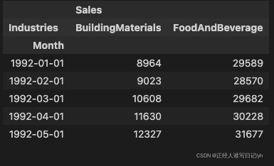
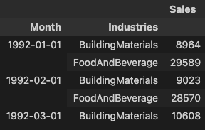
retail = pd.read_csv(
    data_dir / "us-retail-sales.csv",
    usecols=['Month'] + industries,
    parse_dates=['Month'],
    index_col='Month',
).to_period('D').reindex(columns=industries)
retail = pd.concat({'Sales': retail}, names=[None, 'Industries'], axis=1)

retail.head()

首先让我们使用线性回归模型来学习每个系列的趋势。 为了演示，我们将使用二次（2 阶）趋势。 （这里的代码和上一课的代码基本相同。）虽然fit并不完美，但足以满足我们的需要。

y = retail.copy()

# Create trend features
dp = DeterministicProcess(
    index=y.index,  # dates from the training data
    constant=True,  # the intercept
    order=2,        # quadratic trend
    drop=True,      # drop terms to avoid collinearity
)
X = dp.in_sample()  # features for the training data

# Test on the years 2016-2019. It will be easier for us later if we
# split the date index instead of the dataframe directly.
idx_train, idx_test = train_test_split(
    y.index, test_size=12 * 4, shuffle=False,
)
X_train, X_test = X.loc[idx_train, :], X.loc[idx_test, :]
y_train, y_test = y.loc[idx_train], y.loc[idx_test]

y_train

X_train

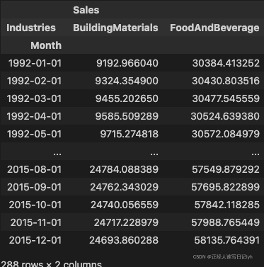
# Fit trend model
model = LinearRegression(fit_intercept=False)
model.fit(X_train, y_train)

# Make predictions
y_fit = pd.DataFrame(
    model.predict(X_train),
    index=y_train.index,
    columns=y_train.columns,
)
y_pred = pd.DataFrame(
    model.predict(X_test),
    index=y_test.index,
    columns=y_test.columns,
)

y_fit

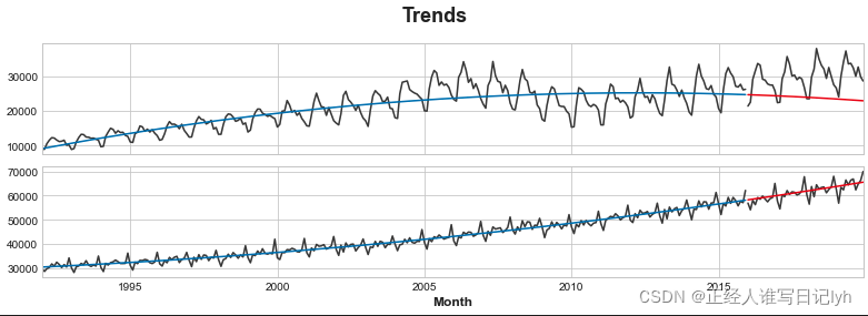
# Plot
axs = y_train.plot(color='0.25', subplots=True, sharex=True)
axs = y_test.plot(color='0.25', subplots=True, sharex=True, ax=axs)
axs = y_fit.plot(color='C0', subplots=True, sharex=True, ax=axs)
axs = y_pred.plot(color='C3', subplots=True, sharex=True, ax=axs)
for ax in axs: ax.legend([])
_ = plt.suptitle("Trends")

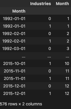
虽然线性回归算法能够进行多输出回归，但 XGBoost 算法却不能。为了使用 XGBoost 一次预测多个系列，我们将把这些系列从 wide 格式（每列一个时间系列）转换为 long 格式，系列按行的类别索引。

# The `stack` method converts column labels to row labels, pivoting from wide format to long
X = retail.stack()  # pivot dataset wide to long
display(X.head())
y = X.pop('Sales')  # grab target series

为了让 XGBoost 能够学会区分我们的两个时间序列，我们将“行业”的行标签转换为带有标签编码的分类特征。 我们还将通过从时间索引中提取月份数字来创建年度季节性特征。

# Turn row labels into categorical feature columns with a label encoding
X = X.reset_index('Industries')
# Label encoding for 'Industries' feature
for colname in X.select_dtypes(["object", "category"]):
    X[colname], _ = X[colname].factorize()

# Label encoding for annual seasonality
X["Month"] = X.index.month  # values are 1, 2, ..., 12

# Create splits
X_train, X_test = X.loc[idx_train, :], X.loc[idx_test, :]
y_train, y_test = y.loc[idx_train], y.loc[idx_test]

X_train 

y_train

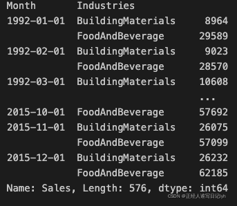
现在我们将之前所做的趋势预测转换为长格式，然后从原始系列中减去它们。 这将为我们提供 XGBoost 可以学习的去趋势（残差）系列。

# Pivot wide to long (stack) and convert DataFrame to Series (squeeze)
y_fit = y_fit.stack().squeeze()    # trend from training set
y_pred = y_pred.stack().squeeze()  # trend from test set

# Create residuals (the collection of detrended series) from the training set
y_resid = y_train - y_fit

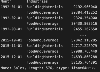
y_fit

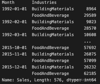
y_train

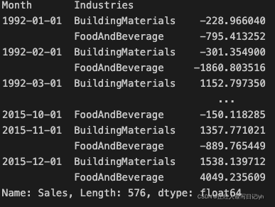
y_resid

# Train XGBoost on the residuals
xgb = XGBRegressor()
xgb.fit(X_train, y_resid)

# Add the predicted residuals onto the predicted trends
y_fit_boosted = xgb.predict(X_train) + y_fit
y_pred_boosted = xgb.predict(X_test) + y_pred

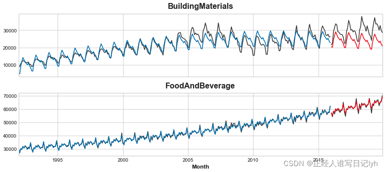
拟合看起来相当不错，尽管我们可以看到 XGBoost 学习的趋势与线性回归学习的趋势一样好 – 特别注意的是 XGBoost 无法弥补'BuildingMaterials'系列中拟合不佳的趋势。

axs = y_train.unstack(['Industries']).plot(
    color='0.25', figsize=(11, 5), subplots=True, sharex=True,
    title=['BuildingMaterials', 'FoodAndBeverage'],
)
axs = y_test.unstack(['Industries']).plot(
    color='0.25', subplots=True, sharex=True, ax=axs,
)
axs = y_fit_boosted.unstack(['Industries']).plot(
    color='C0', subplots=True, sharex=True, ax=axs,
)
axs = y_pred_boosted.unstack(['Industries']).plot(
    color='C3', subplots=True, sharex=True, ax=axs,
)
for ax in axs: ax.legend([])

轮到你了

使用 XGBoost 混合模型预测商店销售额(Forecast Store Sales) 并尝试其他 ML 算法组合。