应用随机过程代码篇 diffusion原理和代码 ode和sde 实验一

引言

目前最新颖又广泛的两种生成式方法是denoising diffusion models and flow matching。这些模型是sota级别的图像、音频和视频生成模型的核心，甚至在google的alphafold3上都有所突出表现。
所有这些生成模型，都是通过将噪声逐步转换为数据来生成对象的。从噪声到数据的这一演变过程是通过模拟常微分方程或随机微分方程来实现的。这里会附上学习的笔记，以及lab的代码和个人的完成，参考课程见文末。

库的引用如下：

from abc import ABC, abstractmethod
from typing import Optional
import math

import numpy as np
from matplotlib import pyplot as plt
from matplotlib.axes._axes import Axes
import torch
import torch.distributions as D
from torch.func import vmap, jacrev
from tqdm import tqdm
import seaborn as sns

device = torch.device('cuda' if torch.cuda.is_available() else 'cpu')

第零部分 起源

来说说几种模式，modalities，比如image，video，molecular structure

1. image，有长宽$H\ast W$，考虑RGB格式，那可以理解为$H\ast W\ast 3$，给定一个image，其在image空间里可以视为$z\in R^{H\ast W\ast 3}$
2. video的话，可以视为一个又一个image在时间轴上的拼接，一秒钟有多少个帧率，那就是多少个图片，比如是T，那么一个视频在video空间内可以视为$z\in R^{H\ast W\ast T\ast 3}$
3. 如果是分子结构，那就要考虑每个分子内的每个原子，去描述这个分子的结构，每个分子是$z^i\in R^3$，可以理解为在三维空间中的一个球（量子概率球90%），如果这个分子有N个原子，就是$z=(z^1,\dots ,z^N)\in R^{3\ast N}$。这只是一个简单描述，更复杂的可以参考Junction Tree Variational Autoencoder for Molecular Graph Generation这篇论文，JTVAE或者MPNN：Neural Message Passing for Quantum Chemistry或者别的更复杂更新颖的方法。

到此我们提炼出一个核心的精要，我们想要生成一个内容，这个内容可以被一个高维的向量空间中的一个展平的向量代替，即$z\in R^d$。以我的理解，生成模型就是去找我们期望的向量附近的和它极度相关的内容，就像是在数学里的邻域去找。不过值得注意的是，上面的例子里没有文本向量，因为自回归模型是离散的。这里主要说明连续数据下的应用。不过二月份arxiv已经有论文LLaDA了，用mask技术把diffusion结合在LLM里，可以自行参考。

ok，再说说“生成”，generate的含义。在机器学习里，我们想要生成一个东西，比如说一个森林风景画，我们考虑生成的是整个森林风景画的一个“条带”，spectrum，生成的风景画和所谓“最好的”风景画会有所区别（没有一个单独的“最好”），有的风景画看着更好，有的看着更差。生成本质上是生成了一个概率分布，如果我们要生成森林风景画，那么我们在“森林风景画”上会给予更高的似然概率。也就是说，我们生成的一个图像，或者视频，或者分子结构，在何种程度上满足一个主观的好坏评价，是被一个$p_{data}$的分布给替代了的。那么生成的任务就是去找这个$p_{data}$，也就是生成了一个目标z，z是采样于分布里的：$z\sim p_{data}$.

生成模型就是这样一个允许我们从$p_{d}ata$里去生成样本的机器学习模型。回想机器学习的三要素，模型，策略，算法，模型想在假设空间里找最优解，我们没有一整个假设空间的信息，只有有限的数据去尝试寻找这个最优解。在生成模型里，有限的数据也就是有限的，从$p_{data}$里取样的数据，也就是$p_1,\dots ,p_N\sim p_{data}$.

很多时候，我们想给定一些数据$y$，去生成一些数据。比如stable diffusion 2022，我们输入positive和negative的prompt，模型就给我们生成在给定文本条件下的图片。这就是从条件分布中的取样：$z\sim p_{data}(\cdot |y)$，y就是条件变量，我们把$p_{data}(\cdot |y)$称呼为条件数据分布，conditional data distribution。条件生成模型，conditional generative modeling在训练过程中一般使用一个随机的，而不是固定的y去训练。然而，事实证明，无条件生成技术很容易推广到条件生成的情况（暂且不表）。因此，文初将完全专注于无条件生成的情况，但要牢记目标是构建条件生成。

那么具体要如何从$p_{data}$生成样本呢？假设我们可以比较容易取样的$p_{init}$，比如高斯分布$p_{init}=\mathcal{N}(0,I_d)$，d就是前面说的样本向量的情况，$z\in R^d$。不过$p_{init}$大可不必和高斯分布一样简单。

总结：

1. 生成的目标就像是$z\in R^d$这样的向量。
2. 生成任务是在训练期间利用一个样本数据集 $z_1,\dots ,z_N\sim p_{\text{data}}$，从概率分布 $p_{\text{data}}$中生成样本。
3. 条件生成假设我们以标签 $y$为条件来确定分布，并且我们希望在训练过程中，利用成对数据集 $(z_1,y)\dots (z_N,y)$从 $p_{\text{data}}(\cdot |y)$中进行采样。
4. 目标是训练一个把样本从$p_{init}$的取样转变为从$p_{data}$取样的生成模型。

第一部分 flow and diffusion models

flow models

一个常微分方程的一个解是通过一个轨迹，trajectory定义的：
$$\begin{array}{c}X:[0,1]\to R^d,t\to X_t\end{array}$$
这个轨迹描绘了从时间$t$到$R^d$某个位置的情况，每个常微分方程都是通过一个向量场，vector field定义的，即如下形式：
$$\begin{array}{c}u:R^d\times [0,1]\to R^d,(x,t)\to u_t(x)\end{array}$$
即，对于每个时间$t$和位置$x$，我们有一个向量$u_t(x)\in R^d$，指定了空间中的一个速度。常微分方程对轨迹施加了一个条件：我们希望轨迹 $X$从点 $x_0$出发，“沿着”向量场 $u_t$ 的方向移动。我们可以将这样的轨迹正式定义为以下方程的解：
$$\begin{array}{rl}\frac{d}{dt}{X}_t& =u_t(X_t)\\ X_0& =x_0\end{array}$$
上述第一个公式就是ODE，说明$X_t$的导数是由$u_t$指定的方向，第二个公式就是初始条件，也就是从时间$t=0$，位置从$x_0$开始。那么，如果从$X_0=x_0$和$t=0$的情况开始，任意时间$t$的情况下$X_t$会是什么样子？flow function说明了这个问题，它是这样的ODE的一种解：
$$\begin{array}{rl}\varphi :R^d\times [0,1]\to & R^d,(x_0,t)\to {\varphi }_t(x_0)\\ \frac{d}{dt}{\varphi }_t(x_0)& =u_t({\varphi }_t(x_0))\\ {\varphi }_0(x_0)& =x_0\end{array}$$
给定一个初始条件，ODE的一个轨迹是通过$X_t={\varphi }_t(x_0)$描述的，从这个视角看，向量场，常微分方程们（ODEs），和flows，在直觉上都是同一种东西的三个不同的描述：向量场定义了解为flows的ODEs。

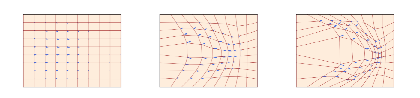
举个例子，这个图片中红色的网格线条就是flow，$u_t$速度场即由蓝色箭头表示，该速度场规定了其在所有位置的瞬时运动，也定义了flow表现的轨迹。随着时间流逝，flow是一个弯曲了$R^2$空间的微分同胚。

一个基本的想法是，对于一个ODE，其解存在吗？存在的话，是否是唯一的呢？从数学上看，存在性和唯一性是满足的，只要满足如下的弱条件假设：如果(2)定义的u是连续可微的，其导数有界，那么(2)中的解通过flow ${\varphi }_t$描述是有唯一解的，在这种情况下，${\varphi }_t$对于所有$t$构成微分同胚映射。这是拓扑学的概念，是一种独特的同胚，也就是说，${\varphi }_t$是连续可微的，它的逆也是。

在机器学习里，这个假设是经常满足的，毕竟神经网络可以用于参数化$u_t(x)$而且导数有界，也就不用担心flows不存在了。

计算ODE

不过一般而言，显式地计算${\varphi }_t$这样的flow是很难的，很多的ODEs都是没有显式解的，所以才有了数值解的说法，也就是利用数值方法，numercial methods，去近似得到ODE的解值。那么ODE的数值方法已经被很多前人探索耕耘过了，比如最简洁浅显的方法，Euler method，通过初始条件$X_0=x_0$，我们如此更新：
$$\begin{array}{c}{X}_{t+h}=X_t+h{u}_t(X_t),t=0,h,2h,\cdots ,1-h\end{array}$$
$h=\frac{1}{n}>0$就是这样的步长超参数，另外还有Heun’s method，有着如下的更新方式：
$$\begin{array}{rl}{X}_{t+h}^{\prime }& =X_t+h{u}_t(x_t),\\ X_{t+h}& =X_t+\frac{h}{2}(u_t(X_t)+u_t(X_{t+h}^{\prime }))\end{array}$$
上面第一个式子是对下一个状态的猜测更新，之后再进行平均，对下一个状态进行实际上的更新。有点像nesterov梯度更新方法的思路。

接下来可以通过一个ODE来构造一个生成模型，注意我们的目的是把一个简单的分布$p_{init}$转化为一个复杂的分布$p_{data}$。
$$\begin{array}{rl}{X}_0& \sim p_{init},\\ \frac{d}{dt}{X}_t& =u_t^{\theta }(X_t)\end{array}$$
这里重磅终于登场，$u_t^{\theta }$就是一个神经网络，有着参数$\theta$，现在开始我们把$u_t^{\theta }$称呼为generic neural network，也就是说，这是一个连续的函数，在参数$\theta$的情况下满足$u_t^{\theta }:R^d\times [0,1]\to R^d$，神经网络的具体选择这里暂且不表，我们的目的是让轨迹的末端$X_1$拥有$p_{data}$这样的分布，也就是：
$$\begin{array}{c}{X}_1\sim p_{data}⟺{\varphi }_1^{\theta }(X_0)\sim p_{data}\end{array}$$
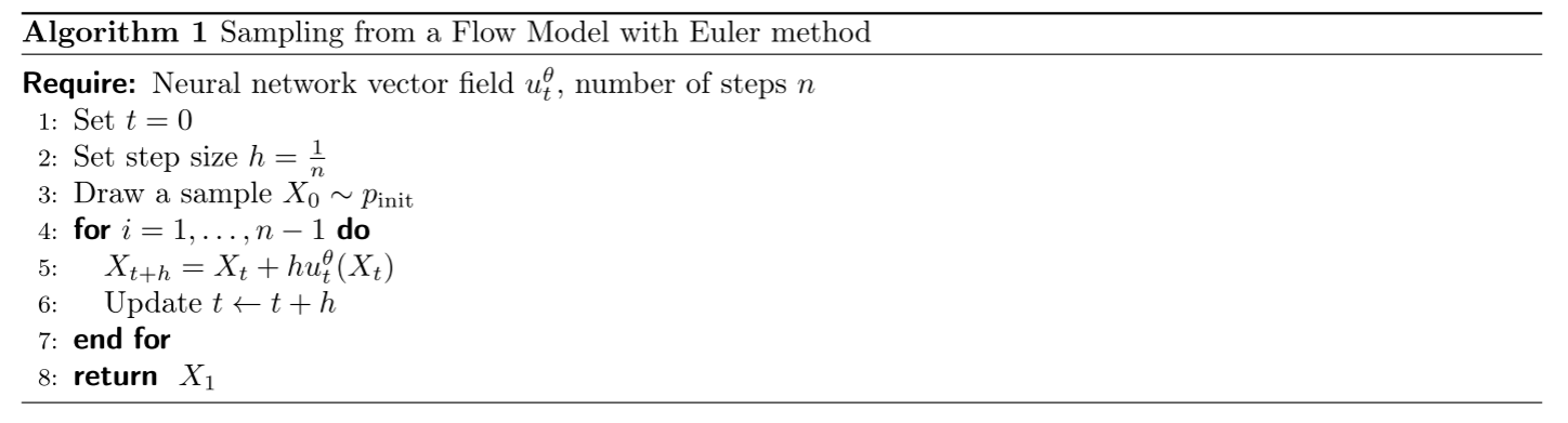
这里，${\varphi }_t^{\theta }$是从 $u_{\theta }(t)$诱导的流。不过请注意：尽管它被称为flow model，但神经网络对向量场进行参数化，而非对流进行参数化。为了计算流，我们需要模拟常微分方程。流模型中采样的过程如下：

diffusion models

随机微分方程，SDEs，延展了像ODEs这样确定性轨迹的方程，使轨迹变得随机起来。一个随机轨迹，stochastic trajectory，被称为是一个随机过程（可以看我上一篇应用随机过程的速通笔记，迅速了解什么是随机过程：应用随机过程笔记1），英文为stochastic process，数学公式写作 { X t , 0 ≤ t ≤ 1 } \{X_t, 0 \le t \le 1\} {Xt​,0≤t≤1}，这里记作$(X_t{)}_{0\le t\le 1}$，式子为：
$$\begin{array}{c}X:[0,1]\to R^d,t\to X_t\end{array}$$
$X_t$在任何一个$t$下是一个随机变量，上面的$t\to X_t$，表示针对每一个$X$都是一个随机轨迹。

Brownian Motion

SDEs是通过布朗运动进行建模的，对于不了解的读者而言可以把它当作一个连续的随机游走，这里给出简洁的说法：一个布朗运动$W=(W(t){)}_{0\le t\le 1}$是一个随机过程，$W_0=0$，轨迹$t\to W_t$是连续的一堆轨迹，而且满足如下两个条件：

1. 增量形式是一个高斯分布，$\forall 0\le s<t,W_t-W_s\sim \mathcal{N}(0,(t-s)I_d)$
2. 增量是独立增量，$\forall t_0,t_1,\cdots ,t_n,s.t.0\le t_0<t_1<\cdots <t_n=1$，$W_{t_1}-W_{t_0},\cdots ,W_{t_n}-W_{t_{n-1}}$都是独立的随机变量（这里注意一下是随机变量，并非一个值）

布朗运动也被称之为Wiener Process，所以其实布朗运动也是一种随机过程，所以布朗运动要给左圈圈右圈圈的数学定义。布朗运动也好建模：
$$\begin{array}{c}{W}_{t+h}=W_t+\sqrt{h}{ϵ}_t,{ϵ}_t\sim \mathcal{N}(0,I_d)(t=0,h,2h,\cdots ,1-h)\end{array}$$

从ODEs到SDEs

从确定性的ODE，延展到有随机性的SDE，是用布朗运动实现的，但是因为随机，无法精确计算到求导式，整个求导过程也是不可以实现的，所以要找不同于求导的表达式。思考刚才的数值方法，以及高等数学的内容，可以做一个变换：
$$\frac{d}{dt}{X}_t=\frac{1}{h}(X_{t+h}-X_t)=u_t(X_t)+R_t(h)⟺X_{t+h}=X_t+h{u}_t(X_t)+h{R}_t(h)$$
$R_t(h)$就是无穷小量，阶数比$u_t$高，可忽略。又想到SDE是ODE的随机性上的延伸，于是在一个极小的$h$上，对上式做出修改：
$$\begin{array}{c}{X}_{t+h}=X_t+h{u}_t(X_t)+{\sigma }_t(W_{t+h}-W_t)+h{R}_t(h)\end{array}$$
这里，${\sigma }_t$就是diffusion coefficient，diffusion的系数，$R_t(h)$是一个随机误差项，在$h\to 0$时满足$\mathbb{E}[\Vert R_t(h{)}^2\Vert {]}^{\frac{1}{2}}\to 0$，上面的式子就刻画了一个随机微分方程，更常见的数学公式表达式这样的：
$$\begin{array}{rl}d{X}_t& =u_t(X_t)dt+{\sigma }_{t}d{W}_t\\ X_0& =x_0\end{array}$$
需要注意的是上面的$d{X}_t$是一种不正式的写法，而且，SDEs再也没有一个flow map ${\varphi }_t$了，因为$X_t$的取值并不是完全取决于$X_0\sim p_{init}$了。
另外，SDE解的存在性和唯一性和之前的ODE一样。ODE（flow model基于此）本身也是一种特殊的SDE，令${\sigma }_t=0$即可。
这里引入一下，标准的SDE右式子是这样的：
$$d{X}_t=f(X_t,t)dt+g(t)d{W}_t$$
左边的$f(X_t,t)dt$是漂移项，drift term，这是确定性的部分，像是一个力场把轨迹朝着某个方向推。在diffusion model里，负责把噪声“推向”数据分布。右边的$g(t)d{W}_t$是扩散项，diffusion term，这就是随机扰动的随即部分了。

计算SDE

和计算ODE差不多，在初始条件$X_0=x_0$时，式子变为
$$\begin{array}{c}{X}_{t+h}=X_t+h{u}_t(X_t)+\sqrt{h}{\sigma }_t{ϵ}_t,{ϵ}_t\sim \mathcal{N}(0,I_d)\end{array}$$
$\sqrt{h}$是怎么来的？回顾布朗运动的增量形式，其服从一个高斯分布，是一个随机变量，高斯分布的标准差是$\Delta W_t\sim \mathcal{N}(0,\Delta t)$，那么提取一下，就是$\Delta W_t=\sqrt{\Delta t}\mathcal{N}(0,I_d)$，也就是说，随机游走的位移和时间的平方根成正比，不是和时间成正比。
算法如下：

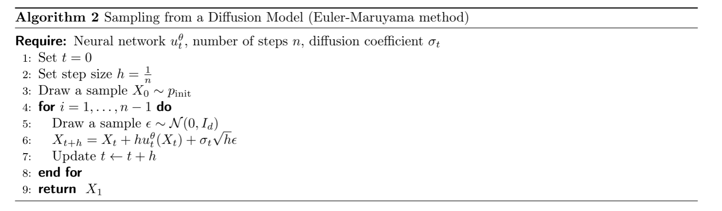
构建生成模型的时候，涉及到神经网络，diffusion model就是这样：
$$\begin{array}{rl}d{X}_t& =u_t^{\theta }(X_t)dt+{\sigma }_{t}d{W}_t\\ X_0& \sim p_{init},\end{array}$$
总结一下，基于SDE的生成模型如此建模：
$$\begin{array}{rl}NeuralNetwork:& u_t^{\theta }:R^d\times [0,1]\to R^d,(x,t)\to u_t^{\theta }(x)\\ Fixed:& {\sigma }_t:[0,1]\to [0,+\infty ),t\to {\sigma }_t\\ Initialization:& X_0\sim p_{init}\\ Simulation:& d{X}_t=u_t^{\theta }(X_t)dt+{\sigma }_{t}d{W}_t\\ Goal:& X_1\sim p_{data}\end{array}$$

代码实验

有了如上的知识，开始编程吧，先编写的是抽象类。

class ODE(ABC):
    @abstractmethod
    def drift_coefficient(self, xt: torch.Tensor, t: torch.Tensor) -> torch.Tensor:
        """
        Returns the drift coefficient of the ODE.
        Args:
            - xt: state at time t, shape (bs, dim)
            - t: time, shape ()
        Returns:
            - drift_coefficient: shape (batch_size, dim)
        """
        pass

class SDE(ABC):
    @abstractmethod
    def drift_coefficient(self, xt: torch.Tensor, t: torch.Tensor) -> torch.Tensor:
        """
        Returns the drift coefficient of the ODE.
        Args:
            - xt: state at time t, shape (batch_size, dim)
            - t: time, shape ()
        Returns:
            - drift_coefficient: shape (batch_size, dim)
        """
        pass

    @abstractmethod
    def diffusion_coefficient(self, xt: torch.Tensor, t: torch.Tensor) -> torch.Tensor:
        """
        Returns the diffusion coefficient of the ODE.
        Args:
            - xt: state at time t, shape (batch_size, dim)
            - t: time, shape ()
        Returns:
            - diffusion_coefficient: shape (batch_size, dim)
        """
        pass

回忆式子(9)和(19)，数值计算模拟的方法可以提取出来一起用，但是每一步更新的方式对于ODE和SDE都是不同的，step方法当作抽象方法待会写。

class Simulator(ABC):
    @abstractmethod
    def step(self, xt: torch.Tensor, t: torch.Tensor, dt: torch.Tensor):
        """
        Takes one simulation step
        Args:
            - xt: state at time t, shape (batch_size, dim)
            - t: time, shape ()
            - dt: time, shape ()
        Returns:
            - nxt: state at time t + dt
        """
        pass

    @torch.no_grad()
    def simulate(self, x: torch.Tensor, ts: torch.Tensor):
        """
        Simulates using the discretization gives by ts
        Args:
            - x_init: initial state at time ts[0], shape (batch_size, dim)
            - ts: timesteps, shape (nts,)
        Returns:
            - x_final: final state at time ts[-1], shape (batch_size, dim)
        """
        for t_idx in range(len(ts) - 1):
            t = ts[t_idx]
            h = ts[t_idx + 1] - ts[t_idx]
            x = self.step(x, t, h)
        return x

    @torch.no_grad()
    def simulate_with_trajectory(self, x: torch.Tensor, ts: torch.Tensor):
        """
        Simulates using the discretization gives by ts
        Args:
            - x_init: initial state at time ts[0], shape (bs, dim)
            - ts: timesteps, shape (num_timesteps,)
        Returns:
            - xs: trajectory of xts over ts, shape (batch_size, num_timesteps, dim)
        """
        xs = [x.clone()]
        for t_idx in tqdm(range(len(ts) - 1)):
            t = ts[t_idx]
            h = ts[t_idx + 1] - ts[t_idx]
            x = self.step(x, t, h)
            xs.append(x.clone())
        return torch.stack(xs, dim=1)

接下来实现Euler方法和Euler-Maruyama方法，前者对应ODE，后者对应SDE：

class EulerSimulator(Simulator):
    def __init__(self, ode: ODE):
        self.ode = ode
        
    def step(self, xt: torch.Tensor, t: torch.Tensor, h: torch.Tensor):
        drift = self.ode.drift_coefficient(xt, t)
        xt_next = xt + h * drift
        
        return xt_next

class EulerMaruyamaSimulator(Simulator):
    def __init__(self, sde: SDE):
        self.sde = sde
        
    def step(self, xt: torch.Tensor, t: torch.Tensor, h: torch.Tensor):
        drift = self.sde.drift_coefficient(xt, t)
        diffusion = self.sde.diffusion_coefficient(xt, t)
        
        #Wiener
        dw = torch.randn_like(xt) * torch.sqrt(h)
        
        xt_next = xt + h * drift + diffusion * dw
        
        return xt_next

布朗过程可以直接看作是：
$$\begin{array}{c}d{X}_t=\sigma d{W}_t,X_0=0\end{array}$$
即在(17)式子里仅保留了随机项。思考当$\sigma$很大和很小的时候轨迹会是什么样子。

class BrownianMotion(SDE):
    def __init__(self, sigma: float):
        self.sigma = sigma
        
    def drift_coefficient(self, xt: torch.Tensor, t: torch.Tensor) -> torch.Tensor:
        """
        Returns the drift coefficient of the ODE.
        Args:
            - xt: state at time t, shape (bs, dim)
            - t: time, shape ()
        Returns:
            - drift: shape (bs, dim)
        """
        drift = torch.zeros_like(xt)
        
        return drift
        
    def diffusion_coefficient(self, xt: torch.Tensor, t: torch.Tensor) -> torch.Tensor:
        """
        Returns the diffusion coefficient of the ODE.
        Args:
            - xt: state at time t, shape (bs, dim)
            - t: time, shape ()
        Returns:
            - diffusion: shape (bs, dim)
        """
        diffusion = torch.full_like(xt, self.sigma)
        
        return diffusion

接下来画图。

def plot_trajectories_1d(x0: torch.Tensor, simulator: Simulator, timesteps: torch.Tensor, ax: Optional[Axes] = None):
        """
        Graphs the trajectories of a one-dimensional SDE with given initial values (x0) and simulation timesteps (timesteps).
        Args:
            - x0: state at time t, shape (num_trajectories, 1)
            - simulator: Simulator object used to simulate
            - t: timesteps to simulate along, shape (num_timesteps,)
            - ax: pyplot Axes object to plot on
        """
        if ax is None:
            ax = plt.gca()
        trajectories = simulator.simulate_with_trajectory(x0, timesteps) # (num_trajectories, num_timesteps, ...)
        for trajectory_idx in range(trajectories.shape[0]):
            trajectory = trajectories[trajectory_idx, :, 0] # (num_timesteps,)
            ax.plot(timesteps.cpu(), trajectory.cpu())

sigma = 1.0
brownian_motion = BrownianMotion(sigma)
simulator = EulerMaruyamaSimulator(sde=brownian_motion)
x0 = torch.zeros(5,1).to(device) # Initial values - let's start at zero
ts = torch.linspace(0.0,5.0,500).to(device) # simulation timesteps

plt.figure(figsize=(8, 8))
ax = plt.gca()
ax.set_title(r'Trajectories of Brownian Motion with $\sigma=$' + str(sigma), fontsize=18)
ax.set_xlabel(r'Time ($t$)', fontsize=18)
ax.set_ylabel(r'$X_t$', fontsize=18)
plot_trajectories_1d(x0, simulator, ts, ax)
plt.show()

这里给一个SDE的例子，Ornstein-Uhlenbeck Process：
在$u_t(X_t)=-\theta X_t$ and ${\sigma }_t=\sigma$情况下：
$$d{X}_t=-\theta X_{t}dt+\sigma d{W}_t,X_0=x_0.$$
思考当$\sigma$很大和很小的时候轨迹会是什么样子。

class OUProcess(SDE):
    def __init__(self, theta: float, sigma: float):
        self.theta = theta
        self.sigma = sigma
        
    def drift_coefficient(self, xt: torch.Tensor, t: torch.Tensor) -> torch.Tensor:
        """
        Returns the drift coefficient of the ODE.
        Args:
            - xt: state at time t, shape (bs, dim)
            - t: time, shape ()
        Returns:
            - drift: shape (bs, dim)
        """
        drift = -self.theta * xt
        
        return drift
        
    def diffusion_coefficient(self, xt: torch.Tensor, t: torch.Tensor) -> torch.Tensor:
        """
        Returns the diffusion coefficient of the ODE.
        Args:
            - xt: state at time t, shape (bs, dim)
            - t: time, shape ()
        Returns:
            - diffusion: shape (bs, dim)
        """
        diffusion = self.sigma * torch.ones_like(xt)        
        return diffusion

两个系数准备完成，接下来开始画图：

# Try comparing multiple choices side-by-side
thetas_and_sigmas = [
    (0.25, 0.0),
    (0.25, 0.25),
    (0.25, 0.5),
    (0.25, 1.0),
]
simulation_time = 20.0

num_plots = len(thetas_and_sigmas)
fig, axes = plt.subplots(1, num_plots, figsize=(8 * num_plots, 7))

for idx, (theta, sigma) in enumerate(thetas_and_sigmas):
    ou_process = OUProcess(theta, sigma)
    simulator = EulerMaruyamaSimulator(sde=ou_process)
    x0 = torch.linspace(-10.0,10.0,10).view(-1,1).to(device) # Initial values - let's start at zero
    ts = torch.linspace(0.0,simulation_time,1000).to(device) # simulation timesteps

    ax = axes[idx]
    ax.set_title(f'Trajectories of OU Process with $\\sigma = ${sigma}, $\\theta = ${theta}', fontsize=15)
    ax.set_xlabel(r'Time ($t$)', fontsize=15)
    ax.set_ylabel(r'$X_t$', fontsize=15)
    plot_trajectories_1d(x0, simulator, ts, ax)
plt.show()

注意根据$D=\frac{{\sigma }^2}{\theta }$这个比率去看轨迹收敛情况，接下来做不同的比率实验，先写一个画图函数。

def plot_scaled_trajectories_1d(x0: torch.Tensor, simulator: Simulator, timesteps: torch.Tensor, time_scale: float, label: str, ax: Optional[Axes] = None):
        """
        Graphs the trajectories of a one-dimensional SDE with given initial values (x0) and simulation timesteps (timesteps).
        Args:
            - x0: state at time t, shape (num_trajectories, 1)
            - simulator: Simulator object used to simulate
            - t: timesteps to simulate along, shape (num_timesteps,)
            - time_scale: scalar by which to scale time
            - label: self-explanatory
            - ax: pyplot Axes object to plot on
        """
        if ax is None:
            ax = plt.gca()
        trajectories = simulator.simulate_with_trajectory(x0, timesteps) # (num_trajectories, num_timesteps, ...)
        for trajectory_idx in range(trajectories.shape[0]):
            trajectory = trajectories[trajectory_idx, :, 0] # (num_timesteps,)
            ax.plot(ts.cpu() * time_scale, trajectory.cpu(), label=label)

# Let's try rescaling with time
sigmas = [1.0, 2.0, 10.0]
ds = [0.25, 1.0, 4.0] # sigma**2 / 2t
simulation_time = 10.0

fig, axes = plt.subplots(len(ds), len(sigmas), figsize=(8 * len(sigmas), 8 * len(ds)))
axes = axes.reshape((len(ds), len(sigmas)))
for d_idx, d in enumerate(ds):
    for s_idx, sigma in enumerate(sigmas):
        theta = sigma**2 / 2 / d
        ou_process = OUProcess(theta, sigma)
        simulator = EulerMaruyamaSimulator(sde=ou_process)
        x0 = torch.linspace(-20.0,20.0,20).view(-1,1).to(device)
        time_scale = sigma**2
        ts = torch.linspace(0.0,simulation_time / time_scale,1000).to(device) # simulation timesteps
        ax = axes[d_idx, s_idx]
        plot_scaled_trajectories_1d(x0=x0, simulator=simulator, timesteps=ts, time_scale=time_scale, label=f'Sigma = {sigma}', ax=ax)
        ax.set_title(f'OU Trajectories with Sigma={sigma}, Theta={theta}, D={d}')
        ax.set_xlabel(f't / (sigma^2)')
        ax.set_ylabel('X_t')
plt.show()

Langevin method给出了一种方法，让任何一个分布都可以从一个简单分布开始表示。根据这个方法的思想，$p_{data}$这个复杂分布是可以从$p_{init}$分布得到的。在实践中，人们可能希望分布具有两种特性：

1. 可以测量分布 $p(x)$ 的密度。这确保我们可以计算对数密度的梯度 $\nabla \log p(x)$ 。这个量被称为 $p$ 的分数，它描绘了分布的局部几何图形。利用该分数，我们将构建并模拟朗之万动力学，可将样本“驱动”向分布 $\pi$ 的方向。特别是，朗温动力学保留了分布$p(x)$。
2. 可以从分布 $p(x)$ 中抽取样本。

对于简单的分布，如高斯分布和简单的混合模型，这两个品质通常都能满足。对于更复杂的 $p$，如图像分布，我们可以采样，但无法测量密度。

class Density(ABC):
    """
    Distribution with tractable density
    """
    @abstractmethod
    def log_density(self, x: torch.Tensor) -> torch.Tensor:
        """
        Returns the log density at x.
        Args:
            - x: shape (batch_size, dim)
        Returns:
            - log_density: shape (batch_size, 1)
        """
        pass

    def score(self, x: torch.Tensor) -> torch.Tensor:
        """
        Returns the score dx log density(x)
        Args:
            - x: (batch_size, dim)
        Returns:
            - score: (batch_size, dim)
        """
        x = x.unsqueeze(1)  # (batch_size, 1, ...)
        #vmap 会为这个函数添加一个批次处理的能力
        #R^{batch_size, dim} -> R^{batch_size, 1}  jacrev: (batch_size, 1, batch_size, dim)
        #vmap每一步，提取一个批次，最后结合成（batch_size, 1, 1, 1, dim)，索引1的1和索引3的1是原batch_size
        score = vmap(jacrev(self.log_density))(x)  # (batch_size, 1, 1, 1, ...)
        #移除索引为 1、2、3 且大小为 1 的维度
        return score.squeeze((1, 2, 3))  # (batch_size, ...)

class Sampleable(ABC):
    """
    Distribution which can be sampled from
    """
    @abstractmethod
    def sample(self, num_samples: int) -> torch.Tensor:
        """
        Returns the log density at x.
        Args:
            - num_samples: the desired number of samples
        Returns:
            - samples: shape (batch_size, dim)
        """
        pass

# Several plotting utility functions
def hist2d_sampleable(sampleable: Sampleable, num_samples: int, ax: Optional[Axes] = None, **kwargs):
    if ax is None:
        ax = plt.gca()
    samples = sampleable.sample(num_samples) # (ns, 2)
    ax.hist2d(samples[:,0].cpu(), samples[:,1].cpu(), **kwargs)

def scatter_sampleable(sampleable: Sampleable, num_samples: int, ax: Optional[Axes] = None, **kwargs):
    if ax is None:
        ax = plt.gca()
    samples = sampleable.sample(num_samples) # (ns, 2)
    ax.scatter(samples[:,0].cpu(), samples[:,1].cpu(), **kwargs)

def imshow_density(density: Density, bins: int, scale: float, ax: Optional[Axes] = None, **kwargs):
    if ax is None:
        ax = plt.gca()
    x = torch.linspace(-scale, scale, bins).to(device)
    y = torch.linspace(-scale, scale, bins).to(device)
    X, Y = torch.meshgrid(x, y)
    xy = torch.stack([X.reshape(-1), Y.reshape(-1)], dim=-1)
    density = density.log_density(xy).reshape(bins, bins).T
    im = ax.imshow(density.cpu(), extent=[-scale, scale, -scale, scale], origin='lower', **kwargs)

def contour_density(density: Density, bins: int, scale: float, ax: Optional[Axes] = None, **kwargs):
    if ax is None:
        ax = plt.gca()
    x = torch.linspace(-scale, scale, bins).to(device)
    y = torch.linspace(-scale, scale, bins).to(device)
    X, Y = torch.meshgrid(x, y)
    xy = torch.stack([X.reshape(-1), Y.reshape(-1)], dim=-1)
    density = density.log_density(xy).reshape(bins, bins).T
    im = ax.contour(density.cpu(), extent=[-scale, scale, -scale, scale], origin='lower', **kwargs)

class Gaussian(torch.nn.Module, Sampleable, Density):
    """
    Two-dimensional Gaussian. Is a Density and a Sampleable. Wrapper around torch.distributions.MultivariateNormal
    """
    def __init__(self, mean, cov):
        """
        mean: shape (2,)
        cov: shape (2,2)
        """
        super().__init__()
        self.register_buffer("mean", mean)
        self.register_buffer("cov", cov)

    @property
    def distribution(self):
        return D.MultivariateNormal(self.mean, self.cov, validate_args=False)

    def sample(self, num_samples) -> torch.Tensor:
        return self.distribution.sample((num_samples,))

    def log_density(self, x: torch.Tensor):
        return self.distribution.log_prob(x).view(-1, 1)

class GaussianMixture(torch.nn.Module, Sampleable, Density):
    """
    Two-dimensional Gaussian mixture model, and is a Density and a Sampleable. Wrapper around torch.distributions.MixtureSameFamily.
    """
    def __init__(
        self,
        means: torch.Tensor,  # nmodes x data_dim
        covs: torch.Tensor,  # nmodes x data_dim x data_dim
        weights: torch.Tensor,  # nmodes
    ):
        """
        means: shape (nmodes, 2)
        covs: shape (nmodes, 2, 2)
        weights: shape (nmodes, 1)
        """
        super().__init__()
        self.nmodes = means.shape[0]
        self.register_buffer("means", means)
        self.register_buffer("covs", covs)
        self.register_buffer("weights", weights)

    @property
    def dim(self) -> int:
        return self.means.shape[1]

    @property
    def distribution(self):
        return D.MixtureSameFamily(
                mixture_distribution=D.Categorical(probs=self.weights, validate_args=False),
                component_distribution=D.MultivariateNormal(
                    loc=self.means,
                    covariance_matrix=self.covs,
                    validate_args=False,
                ),
                validate_args=False,
            )

    def log_density(self, x: torch.Tensor) -> torch.Tensor:
        return self.distribution.log_prob(x).view(-1, 1)

    def sample(self, num_samples: int) -> torch.Tensor:
        return self.distribution.sample(torch.Size((num_samples,)))

    @classmethod
    def random_2D(
        cls, nmodes: int, std: float, scale: float = 10.0, seed = 0.0
    ) -> "GaussianMixture":
        torch.manual_seed(seed)
        means = (torch.rand(nmodes, 2) - 0.5) * scale
        covs = torch.diag_embed(torch.ones(nmodes, 2)) * std ** 2
        weights = torch.ones(nmodes)
        return cls(means, covs, weights)

    @classmethod
    def symmetric_2D(
        cls, nmodes: int, std: float, scale: float = 10.0,
    ) -> "GaussianMixture":
        angles = torch.linspace(0, 2 * np.pi, nmodes + 1)[:nmodes]
        means = torch.stack([torch.cos(angles), torch.sin(angles)], dim=1) * scale
        covs = torch.diag_embed(torch.ones(nmodes, 2) * std ** 2)
        weights = torch.ones(nmodes) / nmodes
        return cls(means, covs, weights)

# Visualize densities
densities = {
    "Gaussian": Gaussian(mean=torch.zeros(2), cov=10 * torch.eye(2)).to(device),
    "Random Mixture": GaussianMixture.random_2D(nmodes=5, std=1.0, scale=20.0, seed=3.0).to(device),
    "Symmetric Mixture": GaussianMixture.symmetric_2D(nmodes=5, std=1.0, scale=8.0).to(device),
}

fig, axes = plt.subplots(1,3, figsize=(18, 6))
bins = 100
scale = 15
for idx, (name, density) in enumerate(densities.items()):
    ax = axes[idx]
    ax.set_title(name)
    imshow_density(density, bins, scale, ax, vmin=-15, cmap=plt.get_cmap('Blues'))
    contour_density(density, bins, scale, ax, colors='grey', linestyles='solid', alpha=0.25, levels=20)
plt.show()

以一个过阻尼langevin dynamics方程做例子：
$$d{X}_t=\frac{1}{2}{\sigma }^2\nabla \log p(X_t)dt+\sigma d{W}_t$$

class LangevinSDE(SDE):
    def __init__(self, sigma: float, density: Density):
        self.sigma = sigma
        self.density = density
        
    def drift_coefficient(self, xt: torch.Tensor, t: torch.Tensor) -> torch.Tensor:
        """
        Returns the drift coefficient of the ODE.
        Args:
            - xt: state at time t, shape (bs, dim)
            - t: time, shape ()
        Returns:
            - drift: shape (bs, dim)
        """
        score = self.density.score(xt)
        drift = 0.5 * self.sigma**2 * score
        return drift
                
    def diffusion_coefficient(self, xt: torch.Tensor, t: torch.Tensor) -> torch.Tensor:
        """
        Returns the diffusion coefficient of the ODE.
        Args:
            - xt: state at time t, shape (bs, dim)
            - t: time, shape ()
        Returns:
            - diffusion: shape (bs, dim)
        """
        diffusion = torch.full_like(xt, self.sigma)
        return diffusion

接下来就可以画图了。

# First, let's define two utility functions...
def every_nth_index(num_timesteps: int, n: int) -> torch.Tensor:
    """
    Compute the indices to record in the trajectory
    """
    if n == 1:
        return torch.arange(num_timesteps)
    return torch.cat(
        [
            torch.arange(0, num_timesteps - 1, n),
            torch.tensor([num_timesteps - 1]),
        ]
    )

def graph_dynamics(
    num_samples: int,
    source_distribution: Sampleable,
    simulator: Simulator, 
    density: Density,
    timesteps: torch.Tensor, 
    plot_every: int,
    bins: int,
    scale: float
):
    """
    Plot the evolution of samples from source under the simulation scheme given by simulator (itself a discretization of an ODE or SDE).
    Args:
        - num_samples: the number of samples to simulate
        - source_distribution: distribution from which we draw initial samples at t=0
        - simulator: the discertized simulation scheme used to simulate the dynamics
        - density: the target density
        - timesteps: the timesteps used by the simulator
        - plot_every: number of timesteps between consecutive plots
        - bins: number of bins for imshow
        - scale: scale for imshow
    """
    # Simulate
    x0 = source_distribution.sample(num_samples)
    xts = simulator.simulate_with_trajectory(x0, timesteps)
    indices_to_plot = every_nth_index(len(timesteps), plot_every)
    plot_timesteps = timesteps[indices_to_plot]
    plot_xts = xts[:,indices_to_plot]

    # Graph
    fig, axes = plt.subplots(2, len(plot_timesteps), figsize=(8*len(plot_timesteps), 16))
    axes = axes.reshape((2,len(plot_timesteps)))
    for t_idx in range(len(plot_timesteps)):
        t = plot_timesteps[t_idx].item()
        xt = xts[:,t_idx]
        # Scatter axes
        scatter_ax = axes[0, t_idx]
        imshow_density(density, bins, scale, scatter_ax, vmin=-15, alpha=0.25, cmap=plt.get_cmap('Blues'))
        scatter_ax.scatter(xt[:,0].cpu(), xt[:,1].cpu(), marker='x', color='black', alpha=0.75, s=15)
        scatter_ax.set_title(f'Samples at t={t:.1f}', fontsize=15)
        scatter_ax.set_xticks([])
        scatter_ax.set_yticks([])

        # Kdeplot axes
        kdeplot_ax = axes[1, t_idx]
        imshow_density(density, bins, scale, kdeplot_ax, vmin=-15, alpha=0.5, cmap=plt.get_cmap('Blues'))
        sns.kdeplot(x=xt[:,0].cpu(), y=xt[:,1].cpu(), alpha=0.5, ax=kdeplot_ax,color='grey')
        kdeplot_ax.set_title(f'Density of Samples at t={t:.1f}', fontsize=15)
        kdeplot_ax.set_xticks([])
        kdeplot_ax.set_yticks([])
        kdeplot_ax.set_xlabel("")
        kdeplot_ax.set_ylabel("")

    plt.show()

# Construct the simulator
target = GaussianMixture.random_2D(nmodes=5, std=0.75, scale=15.0, seed=3.0).to(device)
sde = LangevinSDE(sigma = 10.0, density = target)
simulator = EulerMaruyamaSimulator(sde)

# Graph the results!
graph_dynamics(
    num_samples = 1000,
    source_distribution = Gaussian(mean=torch.zeros(2), cov=20 * torch.eye(2)).to(device),
    simulator=simulator,
    density=target,
    timesteps=torch.linspace(0,5.0,1000).to(device),
    plot_every=334,
    bins=200,
    scale=15
)   

内容和代码参考

MIT Class 6.S184: Generative AI With Stochastic Differential Equations, 2025