deep learning.ai作业：Class 1 Week 2 assignment2_2

Logistic Regression with a Neural Network mindset

Welcome to your first (required) programming assignment! You will build a logistic regression classifier to recognize cats. This assignment will step you through how to do this with a Neural Network mindset, and so will also hone your intuitions about deep learning.

Instructions:

• Do not use loops (for/while) in your code, unless the instructions explicitly ask you to do so.

You will learn to:

• Build the general architecture of a learning algorithm, including:
  • Initializing parameters
  • Calculating the cost function and its gradient
  • Using an optimization algorithm (gradient descent)
• Gather all three functions above into a main model function, in the right order.

 

1 - Packages

First, let's run the cell below to import all the packages that you will need during this assignment.

• numpy is the fundamental package for scientific computing with Python.
• h5py is a common package to interact with a dataset that is stored on an H5 file.
• matplotlib is a famous library to plot graphs in Python.
• PIL and scipy are used here to test your model with your own picture at the end.

import numpy as np
import matplotlib.pyplot as plt
import h5py
import scipy
from PIL import Image
from scipy import ndimage
from lr_utils import load_dataset

%matplotlib inline

2 - Overview of the Problem set

Problem Statement: You are given a dataset ("data.h5") containing:

- a training set of m_train images labeled as cat (y=1) or non-cat (y=0)
- a test set of m_test images labeled as cat or non-cat
- each image is of shape (num_px, num_px, 3) where 3 is for the 3 channels (RGB). Thus, each image is square (height = num_px) and (width = num_px).

You will build a simple image-recognition algorithm that can correctly classify pictures as cat or non-cat.

Let's get more familiar with the dataset. Load the data by running the following code.

# Loading the data (cat/non-cat)
train_set_x_orig, train_set_y, test_set_x_orig, test_set_y, classes = load_dataset()

We added "_orig" at the end of image datasets (train and test) because we are going to preprocess them. After preprocessing, we will end up with train_set_x and test_set_x (the labels train_set_y and test_set_y don't need any preprocessing).

Each line of your train_set_x_orig and test_set_x_orig is an array representing an image. You can visualize an example by running the following code. Feel free also to change the index value and re-run to see other images.

# Example of a picture
index = 25
plt.imshow(train_set_x_orig[index])
print ("y = " + str(train_set_y[:, index]) + ", it's a '" + classes[np.squeeze(train_set_y[:, index])].decode("utf-8") +  "' picture.")

y = [1],it's a cat picture.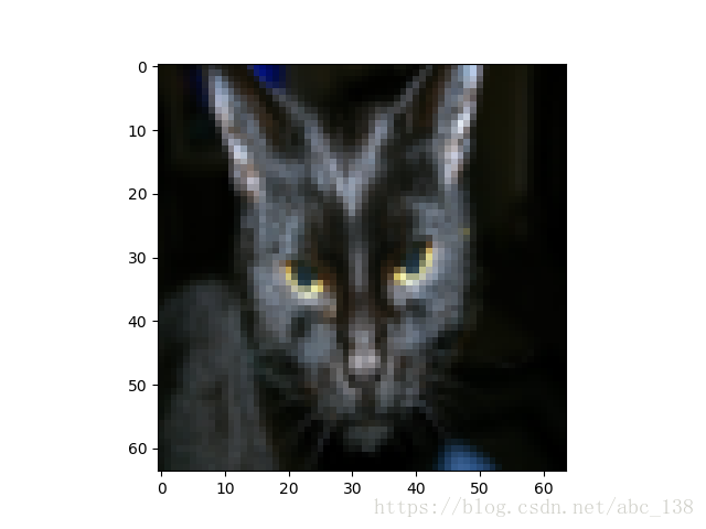

 

Many software bugs in deep learning come from having matrix/vector dimensions that don't fit. If you can keep your matrix/vector dimensions straight you will go a long way toward eliminating many bugs.

Exercise: Find the values for:

- m_train (number of training examples)
- m_test (number of test examples)
- num_px (= height = width of a training image)

Remember that train_set_x_orig is a numpy-array of shape (m_train, num_px, num_px, 3). For instance, you can access m_train by writing train_set_x_orig.shape[0].

m_train = train_set_x_orig.shape[0]
m_test = test_set_x_orig.shape[0]
num_px = train_set_x_orig.shape[1]

print("Number of training example: m_train = " +str(m_train))
print("Number of testing examples: m_test = " + str(m_test))
print("Height/Wight of each image: num_px = " +str(num_px))
print("Each image is of size: (" + str(num_px) + "," + str(num_px) + ",3)")
print("train_set_x shape:" + str(train_set_x_orig.shape))
print("train_set_y shape:" + str(train_set_y.shape))
print("test_set_x shape:" +str(test_set_x_orig.shape))
print("test_set_y shape" + str(test_set_y.shape))

Number of training example: m_train = 209
Number of testing examples: m_test = 50
Height/Wight of each image: num_px = 64
Each image is of size: (64,64,3)
train_set_x shape:(209, 64, 64, 3)
train_set_y shape:(1, 209)
test_set_x shape:(50, 64, 64, 3)
test_set_y shape(1, 50)

For convenience, you should now reshape images of shape (num_px, num_px, 3) in a numpy-array of shape (num_px ∗num_px ∗ 3, 1). After this, our training (and test) dataset is a numpy-array where each column represents a flattened image. There should be m_train (respectively m_test) columns.

Exercise: Reshape the training and test data sets so that images of size (num_px, num_px, 3) are flattened into single vectors of shape (num_px ∗num_px ∗3, 1).

A trick when you want to flatten a matrix X of shape (a,b,c,d) to a matrix X_flatten of shape (b∗c∗d, a) is to use:

X_flatten = X.reshape(X.shape[0], -1).T      # X.T is the transpose of X

# reshape 训练集和测试集
train_set_x_flatten = train_set_x_orig.reshape(m_train,-1).T
test_set_x_flatten = test_set_x_orig.reshape(m_test,-1).T

print("train_set_x_flatten shape: " +str(train_set_x_flatten.shape))
print("train_set_y shape:" + str(train_set_y.shape))
print("test_set_x_flatten shape" + str(test_set_x_flatten.shape))
print("test_set_y shape: " + str(test_set_y.shape))
print("sanity check after reshapeing: " + str(train_set_x_flatten[0:5,0]))

train_set_x_flatten shape: (12288, 209)
train_set_y shape:(1, 209)
test_set_x_flatten shape(12288, 50)
test_set_y shape: (1, 50)
sanity check after reshapeing: [17 31 56 22 33]

To represent color images, the red, green and blue channels (RGB) must be specified for each pixel, and so the pixel value is actually a vector of three numbers ranging from 0 to 255.

One common preprocessing step in machine learning is to center and standardize your dataset, meaning that you substract the mean of the whole numpy array from each example, and then divide each example by the standard deviation of the whole numpy array. But for picture datasets, it is simpler and more convenient and works almost as well to just divide every row of the dataset by 255 (the maximum value of a pixel channel).

Let's standardize our dataset.

train_set_x = train_set_x_flatten / 255
test_set_x = test_set_x_flatten / 255

What you need to remember:

Common steps for pre-processing a new dataset are:

• Figure out the dimensions and shapes of the problem (m_train, m_test, num_px, ...)
• Reshape the datasets such that each example is now a vector of size (num_px * num_px * 3, 1)
• "Standardize" the data

3 - General Architecture of the learning algorithm

It’s time to design a simple algorithm to distinguish cat images from non-cat images.

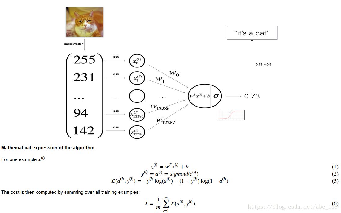
You will build a Logistic Regression, using a Neural Network mindset. The following Figure explains why Logistic Regression is actually a very simple Neural Network!

Key steps:
In this exercise, you will carry out the following steps:
- Initialize the parameters of the model
- Learn the parameters for the model by minimizing the cost
- Use the learned parameters to make predictions (on the test set)
- Analyse the results and conclude

4 - Building the parts of our algorithm

The main steps for building a Neural Network are:

1. Define the model structure (such as number of input features)
2. Initialize the model's parameters
3. Loop:
   • Calculate current loss (forward propagation)
   • Calculate current gradient (backward propagation)
   • Update parameters (gradient descent)

You often build 1-3 separately and integrate them into one function we call model().

4.1 - Helper functions

Exercise: Using your code from "Python Basics", implement sigmoid(). As you've seen in the figure above, you need to compute to make predictions. Use np.exp().

def sigmoid(z):
    s = 1.0 / (1.0 + np.exp(-z))
    return s

print("sigmoid([0,2]) = " + str(sigmoid(np.array([0,2]))))

 

 

 

 

4.2 - Initializing parameters

Exercise: Implement parameter initialization in the cell below. You have to initialize w as a vector of zeros. If you don't know what numpy function to use, look up np.zeros() in the Numpy library's documentation.

def initialize_with_zeros(dim):
    w = np.zeros((dim,1))
    b =0

    assert(w.shape == (dim,1))
    assert(isinstance(b,float) or isinstance(b,int))
    return w,b

 

dim = 2
w, b = initialize_with_zeros(dim)
print ("w = " + str(w))
print ("b = " + str(b))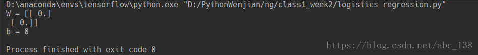

4.3 - Forward and Backward propagation

Now that your parameters are initialized, you can do the "forward" and "backward" propagation steps for learning the parameters.

Exercise: Implement a function propagate() that computes the cost function and its gradient.

 

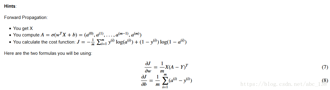
def propagate(w,b,X,Y):
    """
    实现上述传播的成本函数及其梯度

    参数：
     w - 权重，大小不等的数组（num_px * num_px * 3，1）
     b - 偏差，一个标量
     X - 大小数据（num_px * num_px * 3，示例数量）
     Y - 真正的“标签”矢量（包含0如果非猫，1如果猫）的大小（1，例子数）

     返回：
     成本 - 逻辑回归的负对数似然成本
     dw - 相对于w的损失的梯度，因此与w相同的形状
     db - 相对于b的损失梯度，因此与b的形状相同
    
     提示：
     - 为传播逐步编写代码
    """

    m = X.shape[1]
    # 正向传播
    A = sigmoid(np.dot(w.T,X ) + b)
    cost = -(1.0/m)*np.sum(Y*np.log(A) + (1-Y)*np.log(1-A)) # 损失函数
    # 反向传播
    dw = (1.0/m)*np.dot(X,(A-Y).T)
    db = (1.0/m)*np.sum(A-Y)

    assert(dw.shape == w.shape)
    assert(db.dtype == float)
    cost = np.squeeze(cost)
    assert(cost.shape == ())

    grads = {"dw":dw,
             "db":db}
    return grads,cost

 

w,b,X,Y = np.array([[1.],[2.]]),2.,np.array([[1.,2.,-1.],[3.,4.,-3.2]]),np.array([[1,0,1]])
grads, cost = propagate(w,b,X,Y)
print("dw = " + str(grads["dw"]))
print("db = " + str(grads["db"]))
print("cost = " + str(cost))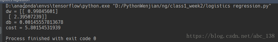

d) Optimization

• You have initialized your parameters.
• You are also able to compute a cost function and its gradient.
• Now, you want to update the parameters using gradient descent.

Exercise: Write down the optimization function. The goal is to learn ww and bb by minimizing the cost function JJ. For a parameter θθ, the update rule is θ=θ−α dθθ=θ−α dθ, where αα is the learning rate.

 

def optimize(w,b,X,Y,num_iterations,learning_rate,print_cost = False):
    """
    此函数通过运行梯度下降算法来优化w和b


    参数：
    w - 权重，大小不等的数组（num_px * num_px * 3，1）
    b - 偏差，一个标量
    X - 形状数据（num_px * num_px * 3，示例数量）
    Y - 真正的“标签”矢量（包含0如果非猫，1如果猫），形状（1，示例数）
    num_iterations - 优化循环的迭代次数
    learning_rate - 梯度下降更新规则的学习率
    print_cost - 每100步打印一次损失


    返回：
    params - 包含权重w和偏差b的字典
    grads - 包含权重和偏差相对于成本函数的梯度的字典
    成本 - 优化期间计算的所有成本列表，这将用于绘制学习曲线。


    提示：
    你基本上需要写下两个步骤并遍历它们：
    1）计算当前参数的成本和梯度。使用propagate（）。
    2）使用w和b的梯度下降法则更新参数。
    """
    costs = []
    for i in range(num_iterations):
        # Cost and gradient calculation
        grads, cost = propagate(w,b,X,Y)

        # Retrieve derivatives from grads
        dw = grads["dw"]
        db = grads["db"]

        # update rule
        w = w - learning_rate * dw
        b = b - learning_rate * db

        # Record the costs
        if i % 100 == 0:
            costs.append(cost)

        # Print the cost every 100 training examples
        if print_cost and i % 100 ==0 :
            print("Cost after iteration %i: %f" %(i ,cost))

    params = {"w":w,"b":b}
    grads = {"dw":dw,"db":db}

    return params,grads,costs

params, grads, costs = optimize(w, b, X, Y, num_iterations= 100, learning_rate = 0.009, print_cost = False)

print ("w = " + str(params["w"]))
print ("b = " + str(params["b"]))
print ("dw = " + str(grads["dw"]))
print ("db = " + str(grads["db"]))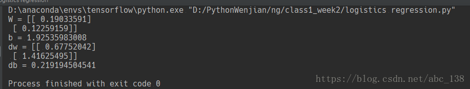

 

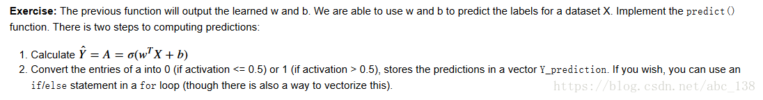
def predict(w,b,X):
    """
    使用学习逻辑回归参数（w，b）预测标签是0还是1，
    
    参数：
     w - 权重，大小不等的数组（num_px * num_px * 3，1）
     b - 偏差，一个标量
     X - 大小数据（num_px * num_px * 3，示例数量）
    
    返回：
     Y_prediction - 包含X中所有例子的所有预测（0/1）的一个numpy数组（向量）
    """
    m = X.shape[1]
    Y_prediction = np.zeros((1,m))
    w = w.reshape(X.shape[0],1)

    #计算向量“A”预测猫在图片中出现的概率
    A = sigmoid(np.dot(w.T,X) + b)

    for i in range (A.shape[1]):

        # 将概率A[0，i]转换为实际预测p[0，i]
        if A[0,i] > 0.5:
            Y_prediction[0,i] = 1
        else:
            Y_prediction[0,i] = 0

    assert (Y_prediction.shape == (1,m))
    return Y_prediction

print("predictions = " +str(predict(w,b,X)))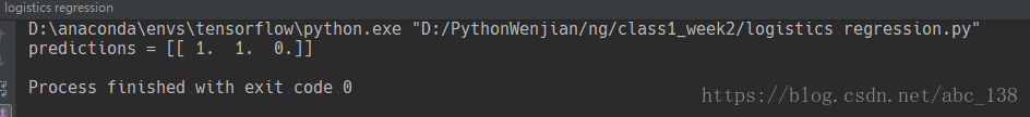

What to remember: You've implemented several functions that:

• Initialize (w,b)
• Optimize the loss iteratively to learn parameters (w,b):
  • computing the cost and its gradient
  • updating the parameters using gradient descent
• Use the learned (w,b) to predict the labels for a given set of examples

 

5 - Merge all functions into a model

You will now see how the overall model is structured by putting together all the building blocks (functions implemented in the previous parts) together, in the right order.

Exercise: Implement the model function. Use the following notation:

- Y_prediction for your predictions on the test set
- Y_prediction_train for your predictions on the train set
- w, costs, grads for the outputs of optimize()

# 执行模型函数

def model(X_train,Y_train,X_test,Y_test,num_iterations = 2000,learning_rate = 0.5,print_cost = False):
    """
    通过调用之前实现的函数来构建逻辑回归模型
    
    参数：
     X_train - 由形状为numpy的数组（num_px * num_px * 3，m_train）表示的训练集
     Y_train - 由形状（1，m_train）的numpy数组（矢量）表示的训练标签
     X_test - 由形状为numpy的数组（num_px * num_px * 3，m_test）表示的测试集
     Y_test - 由形状（1，m_test）的numpy数组（向量）表示的测试标签
     num_iterations - 表示用于优化参数的迭代次数的超参数
     learning_rate - 表示optimize（）更新规则中使用的学习速率的超参数
     print_cost - 设置为true以便每100次迭代打印一次成本
    
    返回：
     d - 包含有关模型信息的字典。
    """
    #用零初始化参数
    w,b = initialize_with_zeros(X_train.shape[0])

    #梯度下降
    parameters,grads,costs = optimize(w,b,X_train,Y_train,num_iterations,learning_rate,print_cost)

    #从字典“参数中检索参数w和b
    w = parameters["w"]
    b = parameters["b"]

    #预测测试/训练集的例子
    Y_prediction_test = predict(w,b,X_test)
    Y_prediction_train = predict(w,b,X_train)

    print("train accuracy: {} %".format(100 - np.mean(np.abs(Y_prediction_train - Y_train)) * 100))
    print("test accuracy: {}%".format(100 - np.mean(np.abs(Y_prediction_test - Y_test)) * 100))

    d = {"costs": costs,
         "Y_prediction_test":Y_prediction_test,
         "Y_prediction_train":Y_prediction_train,
         "w": w,
         "b": b,
         "learning_rate": learning_rate,
         "num_iterations":num_iterations
         }
    return d

 

d = model(train_set_x, train_set_y, test_set_x, test_set_y, num_iterations = 2000, learning_rate = 0.005, print_cost = True)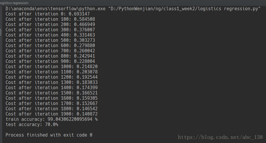

Comment: Training accuracy is close to 100%. This is a good sanity check: your model is working and has high enough capacity to fit the training data. Test error is 68%. It is actually not bad for this simple model, given the small dataset we used and that logistic regression is a linear classifier. But no worries, you'll build an even better classifier next week!

Also, you see that the model is clearly overfitting the training data. Later in this specialization you will learn how to reduce overfitting, for example by using regularization. Using the code below (and changing the index variable) you can look at predictions on pictures of the test set.

# Example of a picture that was wrongly classified.
index = 1
plt.imshow(test_set_x[:,index].reshape((num_px, num_px, 3)))
print ("y = " + str(test_set_y[0,index]) + ", you predicted that it is a \"" + classes[d["Y_prediction_test"][0,index]].decode("utf-8") +  "\" picture.")

 

y = 1, you predicted that it is a "cat" picture.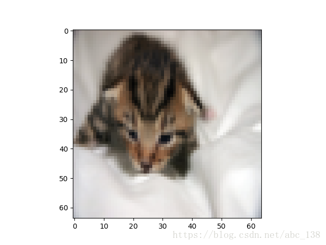

Let's also plot the cost function and the gradients.

# 可视化成本函数和梯度

costs = np.squeeze(d['costs'])
plt.plot(costs)
plt.ylabel('cost')
plt.xlabel('iterations(per hundreds)')
plt.title("Learning rate = " + str(d["learning_rate"]))
plt.show()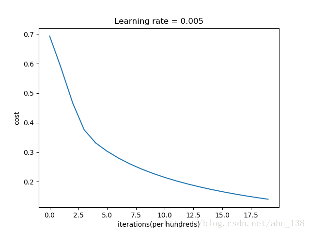

 

Interpretation: You can see the cost decreasing. It shows that the parameters are being learned. However, you see that you could train the model even more on the training set. Try to increase the number of iterations in the cell above and rerun the cells. You might see that the training set accuracy goes up, but the test set accuracy goes down. This is called overfitting.

6 - Further analysis (optional/ungraded exercise)

Congratulations on building your first image classification model. Let's analyze it further, and examine possible choices for the learning rate αα.

Choice of learning rate

Reminder: In order for Gradient Descent to work you must choose the learning rate wisely. The learning rate αα determines how rapidly we update the parameters. If the learning rate is too large we may "overshoot" the optimal value. Similarly, if it is too small we will need too many iterations to converge to the best values. That's why it is crucial to use a well-tuned learning rate.

Let's compare the learning curve of our model with several choices of learning rates. Run the cell below. This should take about 1 minute. Feel free also to try different values than the three we have initialized the learning_rates variable to contain, and see what happens.

learning_rates = [0.01, 0.001, 0.0001]
models = {}
for i in learning_rates:
    print ("learning rate is: " + str(i))
    models[str(i)] = model(train_set_x, train_set_y, test_set_x, test_set_y, num_iterations = 1500, learning_rate = i, print_cost = False)
    print ('\n' + "-------------------------------------------------------" + '\n')

for i in learning_rates:
    plt.plot(np.squeeze(models[str(i)]["costs"]), label= str(models[str(i)]["learning_rate"]))

plt.ylabel('cost')
plt.xlabel('iterations')

legend = plt.legend(loc='upper center', shadow=True)
frame = legend.get_frame()
frame.set_facecolor('0.90')
plt.show()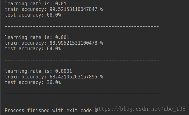

 

 

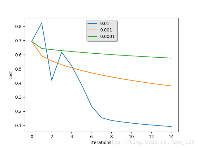
Interpretation:

• Different learning rates give different costs and thus different predictions results.
• If the learning rate is too large (0.01), the cost may oscillate up and down. It may even diverge (though in this example, using 0.01 still eventually ends up at a good value for the cost).
• A lower cost doesn't mean a better model. You have to check if there is possibly overfitting. It happens when the training accuracy is a lot higher than the test accuracy.
• In deep learning, we usually recommend that you:
  • Choose the learning rate that better minimizes the cost function.
  • If your model overfits, use other techniques to reduce overfitting. (We'll talk about this in later videos.)