


 本文深入探讨了机器学习模型的评估与优化方法,包括交叉验证、混淆矩阵、ROC曲线等核心概念,以及如何使用Python的scikit-learn库进行实践。通过实例展示了不同评估指标的计算方式,如准确率、精准率、召回率、F1分数,并介绍了贝叶斯优化器在参数调优中的应用。
文章目录
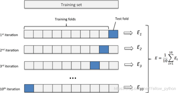
1、交叉验证
- 对原始数据进行分组,训练集(train_set),评估集(valid_set)和测试集(test_set),用训练集对分类器进行训练,再利用评估集来测试训练得到的模型,以选出最优参数组合及对应的模型
1.1、训练集测试集切分
from sklearn.model_selection import train_test_split
X = [11, 22, 33, 44]
y = [10, 20, 30, 40]
X_train, X_test, y_train, y_test = train_test_split(X, y)
print(X_train, X_test, '\n', y_train, y_test)
[44, 11, 22] [33]
[40, 10, 20] [30]
1.2、交叉切分
from sklearn.model_selection import KFold
ls = list('ABC')
kf = KFold(n_splits=3).split(ls)
for i in kf:
    print(i)
(array([1, 2]), array([0]))
(array([0, 2]), array([1]))
(array([0, 1]), array([2]))
1.3、交叉验证结果展示
from sklearn.datasets import make_circles
from sklearn.ensemble import RandomForestClassifier
from sklearn.model_selection import GridSearchCV
import numpy as np, matplotlib.pyplot as mp
np.random.seed(1) # 设定随机环境
X, y = make_circles(n_samples=99, noise=.5, factor=.5) # 创建随机样本
# 交叉验证
clf = RandomForestClassifier() # 随机森林分类器
param = {'min_samples_split': [2, 9], 'max_depth': [4, None]} # 组合参数
model = GridSearchCV(clf, param) # 随机森林分类器+组合参数
model.fit(X, y) # 训练
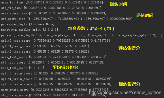
# 交叉验证结果打印
for k, v in model.cv_results_.items():
print(k, v)
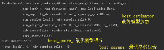
print(model.best_estimator_)
print(model.best_score_)
print(model.best_params_)
- 各模型的训练情况(参数、时间、得分等…)
- 查看最优模型的信息
1.4、贝叶斯定理优化器
from warnings import filterwarnings
filterwarnings('ignore') # 不打印警告
from sklearn.datasets import make_circles
from sklearn.model_selection import train_test_split
from sklearn.svm import SVC
from bayes_opt import BayesianOptimization
import numpy as np
np.random.seed(0)
ls_of_clf = []
def load_data():
X, y = make_circles(n_samples=5000, noise=.3, factor=.4)
X_train, X_test, y_train, y_test = train_test_split(X, y, test_size=.2)
X_train, X_valid, y_train, y_valid = train_test_split(X_train, y_train, test_size=.1)
return X_train, y_train, X_valid, y_valid, X_test, y_test
def score(X_train, y_train, X_valid, y_valid, C):
C = 10 ** C # 幂
clf = SVC(C).fit(X_train, y_train)
ls_of_clf.append(clf)
return clf.score(X_valid, y_valid)
def best_clf(X_train, y_train, X_valid, y_valid):
f = lambda C: score(X_train, y_train, X_valid, y_valid, C)
pbounds = {'C': (-3, 2)} # 取对数使均匀采样【不用(1e-3, 1e2)】
optimizer = BayesianOptimization(f, pbounds)
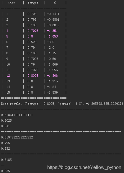
optimizer.maximize(n_iter=10)
print('Best result:', optimizer.max)
idx = optimizer.space.target.argmax()
return ls_of_clf[idx]
X_train, y_train, X_valid, y_valid, X_test, y_test = load_data()
clf = best_clf(X_train, y_train, X_valid, y_valid)
print('--------------------------------------------------------------------')
print(clf.score(X_train, y_train))
print(clf.score(X_valid, y_valid))
print(clf.score(X_test, y_test))
print('--------------------------------------------------------------------')
clf = SVC().fit(X_train, y_train)
print(clf.score(X_train, y_train))
print(clf.score(X_valid, y_valid))
print(clf.score(X_test, y_test))
print('--------------------------------------------------------------------')
X_train = np.concatenate((X_train, X_valid), axis=0)
y_train = np.concatenate((y_train, y_valid), axis=0)
clf = SVC().fit(X_train, y_train)
print(clf.score(X_train, y_train))
print('--')
print(clf.score(X_test, y_test))
2、混淆矩阵
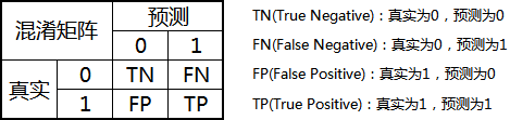
2.1、准确率
A c c u r a c y = C o r r e c t T o t a l = T P + T N T P + T N + F P + F N Accuracy = \frac{Correct}{Total} = \frac{TP+TN}{TP+TN+FP+FN} Accuracy=TotalCorrect=TP+TN+FP+FNTP+TN
2.2、精准率
正确预测1 / 全部预测1
P
r
e
c
i
s
i
o
n
=
T
P
T
P
+
F
N
Precision = \frac{TP}{TP+FN}
Precision=TP+FNTP
2.3、召回率
正确预测1 / 全部正确1
R
e
c
a
l
l
=
T
P
T
P
+
F
P
Recall = \frac{TP}{TP+FP}
Recall=TP+FPTP
2.4、F1 Score
精确率和召回率的一种调和平均
F
1
=
2
×
p
r
e
c
i
s
i
o
n
×
r
e
c
a
l
l
p
r
e
c
i
s
i
o
n
+
r
e
c
a
l
l
F_1 = 2 \times \frac{precision \times recall}{precision + recall}
F1=2×precision+recallprecision×recall
import numpy as np
from sklearn.datasets import make_blobs
from sklearn.model_selection import train_test_split
from sklearn.linear_model import LogisticRegression
from sklearn.metrics import recall_score, precision_score, confusion_matrix
import matplotlib.pyplot as mp
import seaborn
# 创建随机数据
np.random.seed(3)
X, y = make_blobs(centers=2, cluster_std=5)
X_train, X_test, y_train, y_test = train_test_split(X, y, test_size=0.2)
# 建模、训练
model = LogisticRegression()
model.fit(X_train, y_train)
# 模型评估
y_pred = model.predict(X_test)
accuracy = model.score(X_test, y_test)
precision = precision_score(y_test, y_pred)
recall = recall_score(y_test, y_pred)
matrix = confusion_matrix(y_test, y_pred)
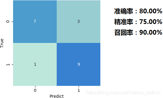
# 结果展示
print('准确率:%.2f%%' % (accuracy * 100))
print('精准率:%.2f%%' % (precision * 100))
print('召回率:%.2f%%' % (recall * 100))
seaborn.heatmap(matrix, center=20, annot=True, cbar=False)
mp.xlabel('Predict')
mp.ylabel('True')
mp.show()
2.5、微平均 & 宏平均
from sklearn.metrics import classification_report
y_true = [1, 1, 2, 2, 0]
y_pred = [1, 0, 2, 2, 0]
print(classification_report(y_true, y_pred))
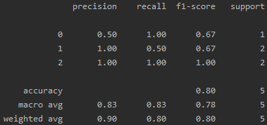
- 宏平均: r e c a l l = 1.00 + 0.50 + 1.00 3 = 0.83 recall = \frac{1.00+0.50+1.00}{3} = 0.83 recall=31.00+0.50+1.00=0.83
- 微平均: r e c a l l = 1.00 × 1 + 0.50 × 2 + 1.00 × 2 5 = 0.8 recall = \frac{1.00 \times 1 + 0.50 \times 2 + 1.00 \times 2 }{5} = 0.8 recall=51.00×1+0.50×2+1.00×2=0.8
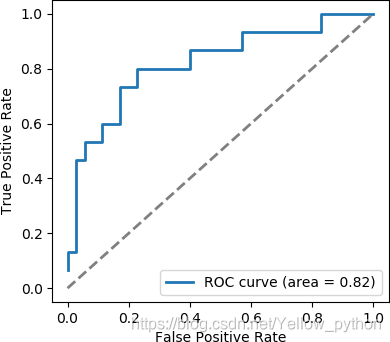
3、ROC
receiver operating characteristic curve:接受者操作特征曲线
import numpy as np, matplotlib.pyplot as mp
from sklearn import svm, datasets
from sklearn.metrics import roc_curve, auc
from sklearn.model_selection import train_test_split
from sklearn.preprocessing import label_binarize
from sklearn.multiclass import OneVsRestClassifier
np.random.seed(0)

"""创建数据"""
X, y = datasets.make_blobs()
# 标签二值化
y = label_binarize(y, classes=[0, 1, 2])  # [0 1 2] -> [[1 0 0][0 1 0][0 0 1]]
n_classes = y.shape[1]
# 对样本添加噪音
n_samples, n_features = X.shape
X = np.c_[X, np.random.randn(n_samples, 200 * n_features)]
# 打乱和切分样本
X_train, X_test, y_train, y_test = train_test_split(X, y, test_size=.5)

"""训练、预测"""
classifier = OneVsRestClassifier(svm.SVC(kernel='linear', probability=True))
y_score = classifier.fit(X_train, y_train).decision_function(X_test)

"""计算每类的【ROC曲线】和【ROC面积】"""
fpr, tpr = dict(), dict()
roc_auc = dict()
for i in range(n_classes):
    fpr[i], tpr[i], thresholds = roc_curve(y_test[:, i], y_score[:, i])  # ROC曲线
    roc_auc[i] = auc(fpr[i], tpr[i])  # ROC面积

"""绘制各类ROC曲线"""
mp.plot(fpr[0], tpr[0], lw=2, label='ROC curve (area = %0.2f) [class0' % roc_auc[0])
mp.plot(fpr[1], tpr[1], lw=2, label='ROC curve (area = %0.2f) [class1' % roc_auc[1])
mp.plot(fpr[2], tpr[2], lw=2, label='ROC curve (area = %0.2f) [class2' % roc_auc[2])
mp.plot([0, 1], [0, 1], color='gray', lw=2, linestyle='--')
mp.xlabel('False Positive Rate')
mp.ylabel('True Positive Rate')
mp.legend(loc='lower right')
mp.show()
4、附录
| En | Cn |
|---|---|
| curve | 曲线 |
| fold | n. 折痕;vt. 折叠 |
| grid search | 格点搜索 |
| ROC | 受试者工作特征曲线 Receiver Operating Characteristic Curve |
| AUC | 曲线下的面积 Area Under Curve |
| False Positive Rate | 假阳性率 |
| True Positive Rate | 真阳性率 |
| negative | 否定;阴性的;消极的 |
| positive | 确定的;阳性的;积极的 |


 4184
4184

 被折叠的 条评论
为什么被折叠?
被折叠的 条评论
为什么被折叠?
 到【灌水乐园】发言


