Python【线性回归】

白手写一个

$$f(x)=wx+b$$
$$loss=(y-(wx+b){)}^2$$
$$\frac{\partial loss}{\partial w}=2x(wx+b-y)$$
$$\frac{\partial loss}{\partial b}=2(wx+b-y)$$

from sklearn.datasets import make_regression
import numpy as np, matplotlib.pyplot as mp

"""创建数据"""
bias = 10.
X, Y, coef = make_regression(n_features=1, noise=9, bias=bias, coef=True)
X = X.reshape(-1)

"""损失值"""
loss = lambda w, b: np.mean([(y - (w * x + b)) ** 2 for x, y in zip(X, Y)])

"""梯度下降"""
def gradient_descent(w, b, lr):
    for x, y in zip(X, Y):
        w -= lr * (((w * x) + b) - y) * x
        b -= lr * (((w * x) + b) - y)
    return w, b

"""运行"""
w, b = .0, .0
for i in range(150, 160):
    print('step%d loss:' % i, loss(w, b))
    w, b = gradient_descent(w, b, 1 / i)  # 渐减的学习率
print(coef, bias, '|', w, b, '|', loss(w, b))

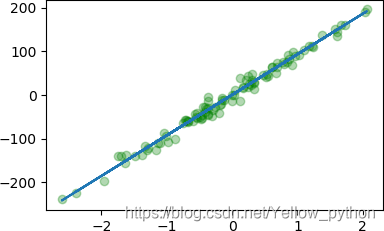
"""可视化"""
mp.scatter(X, Y, c='g', alpha=.3)
mp.plot(X, w * X + b)
mp.show()

调包实现

numpy实现

import numpy as np
# 创建数据
x = [0, 1, 2, 3, 4]
y = [1, 3, 5, 7, 9]
# 斜率、截距
kb = np.polyfit(x, y, 1)
print('y = {:.0f}x + {:.0f}'.format(kb[0], kb[1]))

y = 2x + 1

sklearn实现

import requests, re, numpy as np, matplotlib.pyplot as mp
from mpl_toolkits import mplot3d  # 绘制3d图
from sklearn.linear_model import LinearRegression

# 从网络下载数据
def load_data():
    url = 'https://blog.youkuaiyun.com/Yellow_python/article/details/81224614'
    header = {'User-Agent': 'Opera/8.0 (Windows NT 5.1; U; en)'}
    r = requests.get(url, headers=header)
    data = re.findall('<pre><code>([\s\S]+?)</code></pre>', r.text)[0].strip()
    ndarray = np.array([i.split(',') for i in data.split()]).astype('float')
    return ndarray[:, :2], ndarray[:, -1:]
X, y = load_data()

# 建模、拟合
model = LinearRegression().fit(X, y)
# 系数、截距
k, b = model.coef_[0], model.intercept_[0]

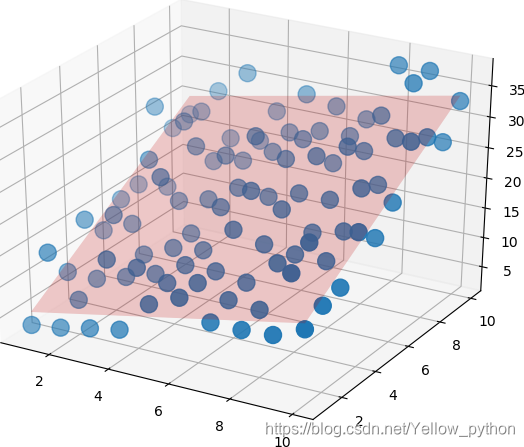
# 可视化
ax = mplot3d.Axes3D(mp.figure())  # 获取三维坐标轴
x1, x2 = X[:, 0], X[:, 1]
ax.scatter(x1, x2, y, s=150)  # 散点图
# 拟合平面
X_predict = np.array([[x1.min(), x2.min()], [x1.min(), x2.max()], [x1.max(), x2.min()]])
X_predict = np.meshgrid(X_predict[:, 0], X_predict[:, 1])
y_predict = X_predict[0] * k[0] + X_predict[1] * k[1] + b
ax.plot_surface(X_predict[0], X_predict[1], y_predict, alpha=0.1, color='red')
mp.show()

TensorFlow实现

https://blog.youkuaiyun.com/Yellow_python/article/details/89108961#_20

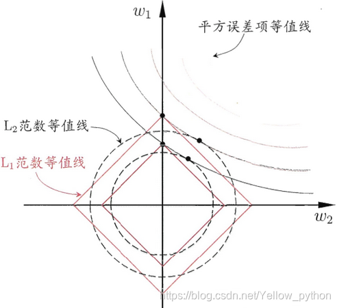
正则化（Regularization）

• L1正则化：
  权值向量w中各个元素的绝对值之和（${\sum }_w|w|$）

• L2正则化：
  权值向量w中各个元素的平方和（${\sum }_w{w}^2$）

• L1正则化和L2正则化可看做是损失函数的【惩罚项】，可使待估参数的偏差变大、方差变小，从而防止过拟合。

Lasso

Least Absolute Shrinkage and Selection Operator
引入L1正则化惩罚，可使某些待估系数收缩到0，比L2更易获得“稀疏解”

Ridge Regression

岭回归
引入L2正则化惩罚，降低过拟合风险

Elastic Net

同时引入L1和L2正则化惩罚

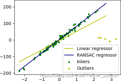
RANSAC

根据一组包含异常数据的样本数据集，计算出数据的数学模型参数，得到有效样本数据。

import numpy as np, matplotlib.pyplot as mp
from sklearn import linear_model, datasets
np.random.seed(1)

"""创建随机样本"""
X, y, coef = datasets.make_regression(n_features=1, noise=9, coef=True)
# 增加异常数据
n_outliers = 5  # 异常值的数量
X[:n_outliers] = 3 + 0.5 * np.random.normal(size=(n_outliers, 1))
y[:n_outliers] = -3 + 10 * np.random.normal(size=n_outliers)

"""建模、拟合"""
# 线性回归
lr = linear_model.LinearRegression().fit(X, y)
# RANSAC（RANdom SAmple Consensus）
ransac = linear_model.RANSACRegressor()
ransac.fit(X, y)
inlier_mask = ransac.inlier_mask_
outlier_mask = np.logical_not(inlier_mask)

"""预测"""
line_X = np.arange(X.min(), X.max())[:, np.newaxis]
line_y = lr.predict(line_X)
line_y_ransac = ransac.predict(line_X)
# 回归系数的比较
print("Estimated coefficients (true, linear regression, RANSAC):")
print(coef, lr.coef_, ransac.estimator_.coef_)

"""可视化"""
mp.scatter(X[inlier_mask], y[inlier_mask], s=9, color='g', label='Inliers')
mp.scatter(X[outlier_mask], y[outlier_mask], s=9, color='y', label='Outliers')
mp.plot(line_X, line_y, color='y', label='Linear regressor')
mp.plot(line_X, line_y_ransac, label='RANSAC regressor')
mp.legend(loc='lower right')
mp.show()

系数更新动态图

from sklearn.datasets import make_regression
import matplotlib.pyplot as mp

"""创建数据"""
X, Y = make_regression(n_features=1, noise=9)
X = X.reshape(-1)

"""参数更新"""
def gradient_descent(w, b, lr):
    for x, y in zip(X, Y):
        w -= lr * (((w * x) + b) - y) * x
        b -= lr * (((w * x) + b) - y)
    return w, b

"""运行过程可视化"""
fig, ax = mp.subplots()
w, b = .0, .0
for i in range(900, 960):
    w, b = gradient_descent(w, b, 1 / i)  # 先大后小的学习率
    ax.cla()  # 清除
    mp.scatter(X, Y, c='g', alpha=.3)  # 散点图
    ax.plot(X, w * X + b)  # 折线图
    mp.pause(1e-9)  # 限时展示

附录

注释

en	cn
coefficient	系数；折算率
intercept	拦截；截距
surface	表面（的）
session	会议；（法庭的）开庭；会话（计算机科学）
optimizer	优化程序
outlier	异常值；局外人
inlier	内围层
shrinkage	n. 收缩
sparse	稀疏

数据源

1,1,3.29
2,1,4.03
3,1,5.12
4,1,6.09
5,1,11.50
6,1,13.74
7,1,10.88
8,1,10.85
9,1,11.24
10,1,13.37
1,2,13.43
2,2,6.68
3,2,14.55
4,2,14.33
5,2,12.97
6,2,14.12
7,2,12.48
8,2,12.08
9,2,19.16
10,2,15.11
1,3,8.23
2,3,8.22
3,3,9.68
4,3,11.33
5,3,13.93
6,3,14.05
7,3,13.34
8,3,17.64
9,3,22.11
10,3,16.00
1,4,15.08
2,4,16.95
3,4,11.46
4,4,13.69
5,4,14.43
6,4,18.91
7,4,17.64
8,4,17.11
9,4,17.15
10,4,22.94
1,5,11.39
2,5,13.58
3,5,22.40
4,5,14.18
5,5,19.62
6,5,23.35
7,5,21.42
8,5,18.73
9,5,20.04
10,5,20.07
1,6,14.77
2,6,22.42
3,6,16.63
4,6,17.98
5,6,20.95
6,6,20.53
7,6,22.16
8,6,22.19
9,6,25.10
10,6,23.90
1,7,15.43
2,7,16.10
3,7,23.87
4,7,23.38
5,7,27.56
6,7,24.89
7,7,26.38
8,7,28.94
9,7,23.83
10,7,31.77
1,8,26.67
2,8,25.21
3,8,19.63
4,8,20.75
5,8,23.24
6,8,26.34
7,8,23.44
8,8,26.45
9,8,29.54
10,8,30.71
1,9,21.37
2,9,25.12
3,9,21.68
4,9,22.28
5,9,24.68
6,9,25.91
7,9,26.09
8,9,30.43
9,9,36.57
10,9,28.16
1,10,21.95
2,10,26.82
3,10,30.76
4,10,25.43
5,10,29.23
6,10,28.23
7,10,27.10
8,10,36.81
9,10,36.86
10,10,33.03