


目录
C. 策略三:压缩因子 (Constriction Factor)
2. 完整进阶代码实现 (Modular Advanced PSO)
1. 二进制粒子群优化 (Binary PSO, BPSO)
1. 引言:从鸟群说起
粒子群优化算法(Particle Swarm Optimization, PSO)是由 Kennedy 和 Eberhart 于 1995 年提出的一种群智能算法。
它的灵感来源于鸟群捕食的行为:一群鸟在随机搜索食物,它们不知道食物在哪里,但它们知道自己当前的位置距离食物有多远,同时也知道整个鸟群中“目前离食物最近的那只鸟”在哪里。
为了找到食物,每只鸟会根据以下三个因素调整自己的飞行速度和方向:
-
惯性:保持之前的飞行状态。
-
个体认知:飞向自己曾经过的最好位置。
-
社会认知:飞向群体目前找到的最好位置。
这种简单的规则涌现出了复杂的群体智能,使得 PSO 成为一种强大的全局优化算法,广泛应用于函数优化、神经网络训练、路径规划等领域。
2. 数学原理

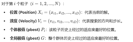
2.1 核心定义
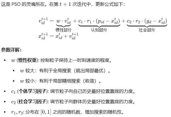
2.2 速度与位置更新公式
3. Python 实现 (向量化版本)
为了提高计算效率,我们不使用循环遍历每个粒子,而是利用 numpy 进行矩阵运算。
import numpy as np

class PSO:
    def __init__(self, func, dim, pop_size=30, max_iter=100, bounds=(-10, 10)):
        """
        :param func: 目标函数 (我们要最小化的函数)
        :param dim: 变量维度
        :param pop_size: 粒子数量
        :param max_iter: 最大迭代次数
        :param bounds: 搜索边界 (min, max)
        """
        self.func = func
        self.dim = dim
        self.pop_size = pop_size
        self.max_iter = max_iter
        self.bounds = bounds

        # PSO 参数 (标准建议值)
        self.w = 0.8      # 惯性权重
        self.c1 = 1.5     # 个体学习因子
        self.c2 = 1.5     # 社会学习因子

        # 初始化粒子位置和速度
        self.X = np.random.uniform(bounds[0], bounds[1], (pop_size, dim))
        self.V = np.random.uniform(-1, 1, (pop_size, dim))

        # 初始化个体最佳 (pbest)
        self.pbest_X = self.X.copy()
        self.pbest_y = self.func(self.X)

        # 初始化全局最佳 (gbest)
        self.gbest_X = np.zeros(dim)
        self.gbest_y = np.inf
        self.update_gbest()

        # 记录历代最优值用于绘图
        self.history = []

    def update_gbest(self):
        """更新全局最优解"""
        min_idx = np.argmin(self.pbest_y)
        if self.pbest_y[min_idx] < self.gbest_y:
            self.gbest_y = self.pbest_y[min_idx]
            self.gbest_X = self.pbest_X[min_idx].copy()

    def run(self):
        for t in range(self.max_iter):
            # 生成随机数矩阵
            r1 = np.random.rand(self.pop_size, self.dim)
            r2 = np.random.rand(self.pop_size, self.dim)

            # --- 核心公式更新 ---
            # 更新速度
            self.V = (self.w * self.V +
                      self.c1 * r1 * (self.pbest_X - self.X) +
                      self.c2 * r2 * (self.gbest_X - self.X))

            # 限制速度 (可选,防止粒子飞太快)
            # self.V = np.clip(self.V, -limit, limit)

            # 更新位置
            self.X = self.X + self.V

            # 边界处理:防止粒子跑出定义域
            self.X = np.clip(self.X, self.bounds[0], self.bounds[1])

            # --- 评估与更新 ---
            # 计算适应度
            y = self.func(self.X)

            # 更新个体最佳 pbest
            # 只有当新位置的适应度比原来的小,才更新
            better_mask = y < self.pbest_y
            self.pbest_X[better_mask] = self.X[better_mask]
            self.pbest_y[better_mask] = y[better_mask]

            # 更新全局最佳 gbest
            self.update_gbest()

            self.history.append(self.gbest_y)

        return self.gbest_X, self.gbest_y, self.history

# --- 测试用例 ---
if __name__ == "__main__":
    # 定义 Sphere 函数: f(x) = x1^2 + x2^2 + ...
    def sphere(x):
        return np.sum(x**2, axis=1)

    pso = PSO(func=sphere, dim=10, pop_size=50, max_iter=100)
    best_x, best_y, history = pso.run()

    print(f"最优解: {best_x}")
    print(f"最优适应度: {best_y}")
进阶粒子群优化:从理论到自适应变种
在标准 PSO 中,参数 $w, c_1, c_2$ 是固定的。这导致了一个致命缺陷:算法在初期“飞得不够散”(容易陷入局部最优),在后期“收敛不够稳”(在最优解附近震荡无法精确)。
为了解决这个问题,学术界提出了多种变种。我们将重点实现三种最经典且行之有效的改进策略:
-
LDIW-PSO (Linear Decreasing Inertia Weight): 线性递减惯性权重。
-
TVAC-PSO (Time-Varying Acceleration Coefficients): 时变加速因子。
-
CF-PSO (Constriction Factor): 压缩因子法(基于特征值分析)。
1. 变种原理深度解析
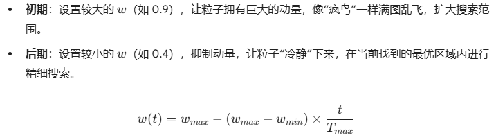
A. 策略一:线性递减权重 (LDIW)
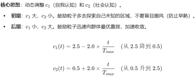
B. 策略二:时变加速因子 (TVAC)
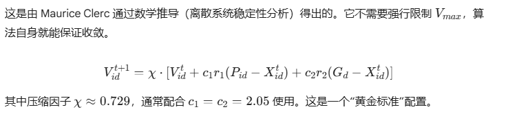
C. 策略三:压缩因子 (Constriction Factor)
2. 完整进阶代码实现 (Modular Advanced PSO)
为了方便实验,我编写了一个模块化的类 AdvancedPSO,你可以在实例化时通过 mode 参数自由切换变种。
此外,为了验证变种的有效性,我们使用 Rastrigin 函数。这是一个高度非凸的函数,充满了成千上万个局部陷阱,标准 PSO 很容易挂在这里,而改进版表现会好很多。
Python
import numpy as np
import matplotlib.pyplot as plt

# ==========================================
# 1. 测试函数:Rastrigin Function
# (非常难的函数,有大量局部最优,全局最优在 0)
# ==========================================
def rastrigin(X):
    # f(x) = 10*d + sum(x_i^2 - 10*cos(2*pi*x_i))
    A = 10
    d = X.shape[1]
    return A * d + np.sum(X**2 - A * np.cos(2 * np.pi * X), axis=1)

# ==========================================
# 2. 进阶 PSO 框架
# ==========================================
class AdvancedPSO:
    def __init__(self, func, dim, pop_size=50, max_iter=200, bounds=(-5.12, 5.12), mode='tvac'):
        """
        :param mode: 算法模式
                     'standard' - 标准 PSO
                     'ldiw'     - 线性递减权重
                     'tvac'     - 时变加速因子 (推荐)
                     'constriction' - 压缩因子法 (Clerc Type 1)
        """
        self.func = func
        self.dim = dim
        self.pop_size = pop_size
        self.max_iter = max_iter
        self.bounds = bounds
        self.mode = mode

        # --- 初始化粒子 ---
        self.X = np.random.uniform(bounds[0], bounds[1], (pop_size, dim))
        # 速度初始化通常为搜索范围的 10%-20%
        v_limit = (bounds[1] - bounds[0]) * 0.2
        self.V = np.random.uniform(-v_limit, v_limit, (pop_size, dim))

        # --- 历史最佳 ---
        self.pbest_X = self.X.copy()
        self.pbest_y = self.func(self.X)

        self.gbest_X = np.zeros(dim)
        self.gbest_y = np.inf
        self.update_gbest()

        self.history = [] # 记录收敛曲线

    def update_gbest(self):
        min_idx = np.argmin(self.pbest_y)
        if self.pbest_y[min_idx] < self.gbest_y:
            self.gbest_y = self.pbest_y[min_idx]
            self.gbest_X = self.pbest_X[min_idx].copy()

    def get_parameters(self, t):
        """
        根据当前迭代次数 t 和选择的 mode,动态计算 w, c1, c2
        """
        # 进度比率 (0 -> 1)
        ratio = t / self.max_iter

        if self.mode == 'standard':
            return 0.7, 1.5, 1.5

        elif self.mode == 'ldiw':
            # w 线性递减: 0.9 -> 0.4
            w = 0.9 - 0.5 * ratio
            return w, 1.5, 1.5

        elif self.mode == 'tvac':
            # w 线性递减
            w = 0.9 - 0.5 * ratio
            # c1 (自我) 递减: 2.5 -> 0.5 (初期多探索自己)
            c1 = 2.5 - 2.0 * ratio
            # c2 (社会) 递增: 0.5 -> 2.5 (后期多跟从群体)
            c2 = 0.5 + 2.0 * ratio
            return w, c1, c2

        elif self.mode == 'constriction':
            # 压缩因子模式:w 实际上就是 chi (压缩因子)
            # 理论值: phi = 4.1, chi = 0.729
            phi = 2.05 + 2.05
            chi = 2 / np.abs(2 - phi - np.sqrt(phi**2 - 4*phi))
            return chi, 2.05, 2.05

        return 0.7, 1.5, 1.5

    def run(self):
        print(f"Starting PSO [Mode: {self.mode}]")

        for t in range(self.max_iter):
            # 1. 获取动态参数
            w, c1, c2 = self.get_parameters(t)

            # 2. 生成随机数
            r1 = np.random.rand(self.pop_size, self.dim)
            r2 = np.random.rand(self.pop_size, self.dim)

            # 3. 更新速度
            # 如果是压缩因子模式,公式略有不同 (乘在最外面)
            if self.mode == 'constriction':
                self.V = w * (self.V +
                              c1 * r1 * (self.pbest_X - self.X) +
                              c2 * r2 * (self.gbest_X - self.X))
            else:
                self.V = (w * self.V +
                          c1 * r1 * (self.pbest_X - self.X) +
                          c2 * r2 * (self.gbest_X - self.X))

            # 4. 更新位置
            self.X = self.X + self.V

            # 边界处理 (Clip)
            self.X = np.clip(self.X, self.bounds[0], self.bounds[1])

            # 5. 计算适应度
            y = self.func(self.X)

            # 6. 更新 Pbest
            better_mask = y < self.pbest_y
            self.pbest_X[better_mask] = self.X[better_mask]
            self.pbest_y[better_mask] = y[better_mask]

            # 7. 更新 Gbest
            self.update_gbest()
            self.history.append(self.gbest_y)

        return self.gbest_y, self.history

# ==========================================
# 3. 对比实验与绘图
# ==========================================
if __name__ == "__main__":
    # 实验设置
    DIM = 30           # 30维 Rastrigin 问题 (很难!)
    POP = 50
    ITER = 500

    # 运行三种不同模式进行对比
    modes = ['standard', 'ldiw', 'tvac', 'constriction']
    results = {}

    plt.figure(figsize=(10, 6))

    for mode in modes:
        # 为了公平,每种模式运行 10 次取平均,减少随机性影响
        avg_history = np.zeros(ITER)
        runs = 10

        print(f"\nTesting {mode}...")
        for _ in range(runs):
            optimizer = AdvancedPSO(rastrigin, DIM, POP, ITER, bounds=(-5.12, 5.12), mode=mode)
            _, hist = optimizer.run()
            avg_history += np.array(hist)

        avg_history /= runs
        results[mode] = avg_history[-1]

        # 绘图
        plt.plot(avg_history, label=f"{mode} (Final: {avg_history[-1]:.2e})")

    plt.title(f'Comparison of PSO Variants on {DIM}-D Rastrigin Function')
    plt.xlabel('Iteration')
    plt.ylabel('Fitness (Log Scale)')
    plt.yscale('log')
    plt.legend()
    plt.grid(True, which="both", ls="-", alpha=0.5)
    plt.show()

    # 打印最终对比
    print("\n=== Final Results (Lower is Better) ===")
    for m, res in results.items():
        print(f"{m.ljust(15)}: {res:.10f}")
3. 代码与结果分析
运行结果预期
当你运行这段代码时,你会清楚地看到不同变种的性能差异(特别是在 30 维 Rastrigin 这种复杂函数上):
-
Standard (标准版):
-
通常表现最差。曲线下降一段后会变成一条水平线。这说明粒子群**“早熟”**了,它们过早地聚集在了一个局部坑里,再也跳不出来了。
-
-
LDIW (线性递减权重):
-
表现优于标准版。曲线下降得更深,说明它在后期进行了更精细的搜索,但可能仍然无法跳出深层的局部最优。
-
-
TVAC (时变加速因子):
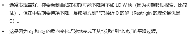
-
Constriction (压缩因子):
-
表现非常稳定,收敛速度通常很快,属于“性价比”极高的选择,不需要复杂的参数调整。
-
二进制粒子群优化 (Binary PSO, BPSO)
应用场景:用于离散问题,如特征选择、背包问题、任务分配(解只能是 0 或 1)。
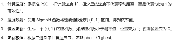
算法步骤
Python 实现代码
import numpy as np

class BinaryPSO:
    def __init__(self, func, dim, pop_size=30, max_iter=100):
        self.func = func
        self.dim = dim
        self.pop_size = pop_size
        self.max_iter = max_iter

        # 初始化位置 (0 或 1)
        self.X = np.random.randint(2, size=(pop_size, dim))
        # 初始化速度
        self.V = np.random.uniform(-1, 1, (pop_size, dim))

        # 初始化极值
        self.pbest_X = self.X.copy()
        self.pbest_score = self.func(self.X)

        self.gbest_X = self.pbest_X[np.argmin(self.pbest_score)].copy()
        self.gbest_score = np.min(self.pbest_score)

        # Sigmoid 函数
        self.sigmoid = lambda x: 1 / (1 + np.exp(-x))

    def run(self):
        print("Starting BPSO...")
        for t in range(self.max_iter):
            # 1. 计算速度 (标准公式)
            r1, r2 = np.random.rand(2)
            self.V = (self.V +
                      1.5 * r1 * (self.pbest_X - self.X) +
                      1.5 * r2 * (self.gbest_X - self.X))

            # 2. 速度映射为概率 (Sigmoid)
            prob = self.sigmoid(self.V)

            # 3. 位置更新 (根据概率决定是 0 还是 1)
            # 生成随机矩阵,如果 rand < prob,则设为 1,否则 0
            rand_matrix = np.random.rand(self.pop_size, self.dim)
            self.X = (rand_matrix < prob).astype(int)

            # 4. 计算适应度
            scores = self.func(self.X)

            # 5. 更新 pbest
            better_mask = scores < self.pbest_score
            self.pbest_X[better_mask] = self.X[better_mask]
            self.pbest_score[better_mask] = scores[better_mask]

            # 6. 更新 gbest
            current_best_val = np.min(self.pbest_score)
            if current_best_val < self.gbest_score:
                self.gbest_score = current_best_val
                self.gbest_X = self.pbest_X[np.argmin(self.pbest_score)].copy()

            print(f"Iter {t}: Best Score = {self.gbest_score}")

# --- 测试用例 (OneMax 问题: 让所有位都变成 1) ---
# 目标函数:返回 0 的个数 (越少越好)
def objective_function(x):
    # x 是 0/1 矩阵,我们希望 1 越多越好,所以最小化 (dim - sum)
    return x.shape[1] - np.sum(x, axis=1)

if __name__ == "__main__":
    bpso = BinaryPSO(objective_function, dim=20, pop_size=30, max_iter=50)
    bpso.run()
量子行为粒子群 (QPSO)
应用场景:这是一种现代变种。它完全抛弃了“速度”向量,认为粒子具有量子行为,出现在某一点是概率性的。它的参数更少,收敛能力通常强于标准 PSO。
算法步骤
-
计算平均最优位置 (mbest):计算群体中所有粒子个体历史最优位置 (pbest) 的平均值。
-
计算局部吸引点 (attractor):对于每个粒子,在它的 pbest 和群体的 gbest 之间随机找一个点作为吸引点。
-
位置更新:根据量子力学的波函数推导,位置由吸引点、平均最优位置和一个收缩扩张系数 (alpha) 决定。粒子直接“瞬移”到新位置。
Python 实现代码
import numpy as np

class QPSO:
    def __init__(self, func, dim, pop_size=30, max_iter=100, bounds=(-10, 10)):
        self.func = func
        self.dim = dim
        self.pop_size = pop_size
        self.max_iter = max_iter
        self.bounds = bounds

        self.X = np.random.uniform(bounds[0], bounds[1], (pop_size, dim))

        # QPSO 没有速度 V

        self.pbest_X = self.X.copy()
        self.pbest_score = self.func(self.X)

        self.gbest_X = self.pbest_X[np.argmin(self.pbest_score)].copy()
        self.gbest_score = np.min(self.pbest_score)

    def run(self):
        print("Starting QPSO...")
        for t in range(self.max_iter):
            # Alpha: 收缩扩张系数,通常从 1.0 线性递减到 0.5
            alpha = 1.0 - 0.5 * (t / self.max_iter)

            # 1. 计算 mbest (Mean Best Position)
            # 所有 pbest 的中心点
            mbest = np.mean(self.pbest_X, axis=0)

            # 2. 更新每个粒子的位置
            # 生成随机数 phi, u
            phi = np.random.rand(self.pop_size, self.dim)
            u = np.random.rand(self.pop_size, self.dim)

            # 计算局部吸引点 p
            # p = phi * pbest + (1-phi) * gbest
            p = phi * self.pbest_X + (1 - phi) * self.gbest_X

            # 核心更新公式 (根据 u > 0.5 分正负)
            # X = p +/- alpha * |mbest - X| * ln(1/u)
            sign = np.where(np.random.rand(self.pop_size, self.dim) > 0.5, 1, -1)

            self.X = p + sign * alpha * np.abs(mbest - self.X) * np.log(1 / u)

            # 边界处理
            self.X = np.clip(self.X, self.bounds[0], self.bounds[1])

            # 3. 更新极值 (同标准 PSO)
            scores = self.func(self.X)
            better_mask = scores < self.pbest_score
            self.pbest_X[better_mask] = self.X[better_mask]
            self.pbest_score[better_mask] = scores[better_mask]

            min_val = np.min(self.pbest_score)
            if min_val < self.gbest_score:
                self.gbest_score = min_val
                self.gbest_X = self.pbest_X[np.argmin(self.pbest_score)].copy()

            if t % 10 == 0:
                print(f"Iter {t}: Best Score = {self.gbest_score:.6f}")

# --- 测试用例 (Sphere 函数) ---
def sphere(x):
    return np.sum(x**2, axis=1)

if __name__ == "__main__":
    qpso = QPSO(sphere, dim=10, pop_size=40, max_iter=100)
    qpso.run()


 1724
1724

 被折叠的 条评论
为什么被折叠?
被折叠的 条评论
为什么被折叠?
 到【灌水乐园】发言


