import numpy as np
import matplotlib.pyplot as plt
from mpl_toolkits.mplot3d import Axes3D
from matplotlib.collections import PolyCollection
import os
import matplotlib.tri as mtri
from datetime import datetime
from geometry_processor import *
plt.rcParams["font.family"] = ["SimHei", "WenQuanYi Micro Hei", "Heiti TC"]
plt.rcParams["axes.unicode_minus"] = False
plt.rcParams["font.family"] = ["SimHei", "WenQuanYi Micro Hei", "Heiti TC", "Arial Unicode MS"]
class FlowVisualizer:
"""流场可视化器"""
def __init__(self):
self.geometry = None
self.results = None
self.flow_conditions = None
self.config = None
self.view_type = 'top' # 默认顶视图
self.analysis_log = [] # 存储日志
def setup(self, geometry, results, flow_conditions, config):
"""初始化可视化器参数"""
self.geometry = geometry
self.results = results
self.flow_conditions = flow_conditions
self.config = config
return self
def logger(self, message):
"""日志记录方法,修复缺失的logger属性"""
timestamp = datetime.now().strftime("%H:%M:%S")
log_entry = f"[{timestamp}] {message}"
print(log_entry) # 打印到控制台
self.analysis_log.append(log_entry) # 保存到日志列表
def plot_geometry_overview(self):
"""绘制几何体总览"""
fig = plt.figure(figsize=(15, 10))
# 3D视图
ax1 = fig.add_subplot(221, projection='3d')
self._plot_3d_geometry(ax1)
# 顶视图
ax2 = fig.add_subplot(222)
self._plot_2d_projection(ax2, 'top')
# 侧视图
ax3 = fig.add_subplot(223)
self._plot_2d_projection(ax3, 'side')
# 前视图
ax4 = fig.add_subplot(224)
self._plot_2d_projection(ax4, 'front')
plt.tight_layout()
if self.config.get('save_figures', False):
plt.savefig('geometry_overview.png', dpi=self.config.get('dpi', 300), bbox_inches='tight')
if self.config.get('auto_show', True):
plt.show()
def _plot_3d_geometry(self, ax):
"""绘制3D几何体(修正3D顶点转2D的问题)"""
# 采样显示面元(避免过于密集)
max_faces = 5000
step = max(1, len(self.geometry.elements) // max_faces)
sample_elements = self.geometry.elements[::step]
# 存储2D面片和对应的z坐标
faces_2d = [] # 2D顶点(X-Y投影)
z_coords = [] # 每个面片的平均z坐标(用于3D定位)
for elem in sample_elements:
# 获取3D顶点(形状为 (N, 3),N为面元顶点数,如三角形为3,四边形为4)
vertices_3d = self.geometry.nodes[elem]
# 将3D顶点投影到X-Y平面(提取x和y作为2D坐标)
vertices_2d = vertices_3d[:, :2] # 取前两列(x, y)
faces_2d.append(vertices_2d)
# 计算该面元的平均z坐标(用于在3D空间中定位面片)
avg_z = np.mean(vertices_3d[:, 2]) # 取z坐标的平均值
z_coords.append(avg_z)
# 创建2D面片集合(此时输入为2D顶点,符合要求)
face_collection = PolyCollection(
faces_2d,
alpha=0.3,
facecolor='lightblue',
edgecolor='darkblue',
linewidth=0.1
)
# 将2D面片添加到3D轴,并通过zs指定每个面片的z坐标
ax.add_collection3d(face_collection, zs=z_coords, zdir='z')
# 设置坐标轴范围
bounds = self.geometry.get_bounds()
ax.set_xlim(bounds[0])
ax.set_ylim(bounds[1])
ax.set_zlim(bounds[2])
ax.set_xlabel('X')
ax.set_ylabel('Y')
ax.set_zlabel('Z')
ax.set_title('3D几何体')
# 设置视角
ax.view_init(elev=20, azim=45)
def _plot_2d_projection(self, ax, view_type):
"""绘制2D投影"""
nodes = self.geometry.nodes
if view_type == 'top': # X-Y平面
x, y = nodes[:, 0], nodes[:, 1]
xlabel, ylabel = 'X (长度)', 'Y (宽度)'
title = '顶视图 (X-Y)'
elif view_type == 'side': # X-Z平面
x, y = nodes[:, 0], nodes[:, 2]
xlabel, ylabel = 'X (长度)', 'Z (高度)'
title = '侧视图 (X-Z)'
else: # 'front' Y-Z平面
x, y = nodes[:, 1], nodes[:, 2]
xlabel, ylabel = 'Y (宽度)', 'Z (高度)'
title = '前视图 (Y-Z)'
ax.scatter(x, y, s=0.5, alpha=0.6, c='blue')
ax.set_xlabel(xlabel)
ax.set_ylabel(ylabel)
ax.set_title(title)
ax.set_aspect('equal')
ax.grid(True, alpha=0.3)
def plot_pressure_distribution(self):
"""绘制压力分布,增强版坐标与数据的匹配逻辑"""
try:
# 获取压力系数数据
if 'shock_expansion' in self.results:
pressure_data = self.results['shock_expansion']['element_data']['pressure_coefficients']
data_source = "激波修正后"
else:
pressure_data = self.results['flow_field']['pressure_coefficients']
data_source = "基本流场"
# 严格匹配逻辑
if len(pressure_data) == len(self.geometry.face_centers):
coords = self.geometry.face_centers # 使用面元中心坐标
self.logger("使用面元中心坐标")
elif len(pressure_data) == len(self.geometry.nodes):
coords = self.geometry.nodes # 使用节点坐标
self.logger("使用节点坐标")
else:
# 自动选择最接近的坐标集
if abs(len(pressure_data) - len(self.geometry.face_centers)) < abs(
len(pressure_data) - len(self.geometry.nodes)):
coords = self.geometry.face_centers
else:
coords = self.geometry.nodes
self.logger(
f"警告: 数据长度不匹配,使用替代坐标 (数据长度={len(pressure_data)}, 坐标长度={len(coords)})")
# 投影到2D视图
if self.view_type == 'top':
x, y = coords[:, 0], coords[:, 1]
xlabel, ylabel = 'X坐标', 'Y坐标'
elif self.view_type == 'side':
x, y = coords[:, 0], coords[:, 2]
xlabel, ylabel = 'X坐标', 'Z坐标'
else:
x, y = coords[:, 1], coords[:, 2]
xlabel, ylabel = 'Y坐标', 'Z坐标'
# 确保数据长度一致
min_length = min(len(x), len(pressure_data))
x = x[:min_length]
y = y[:min_length]
pressure_data = pressure_data[:min_length]
# 绘制压力云图
fig, ax = plt.subplots(figsize=(10, 8))
scatter = ax.scatter(x, y, c=pressure_data, cmap='jet', s=10, alpha=0.8)
plt.colorbar(scatter, ax=ax, label=f'压力系数 ({data_source})')
ax.set_xlabel(xlabel)
ax.set_ylabel(ylabel)
ax.set_title(f'表面压力系数分布 (Ma={self.flow_conditions["mach_number"]})')
ax.set_aspect('equal')
if self.config["save_figures"]:
self._save_figure(fig, "pressure_distribution")
if self.config["auto_show"]:
plt.show()
else:
plt.close(fig)
except Exception as e:
self.logger(f"❌ 压力分布可视化失败: {str(e)}")
# 输出详细调试信息
if hasattr(self, 'geometry'):
self.logger(f"调试信息: 节点数={len(self.geometry.nodes)}, 面元数={len(self.geometry.elements)}")
if hasattr(self.geometry, 'face_centers'):
self.logger(f"面元中心数={len(self.geometry.face_centers)}")
if 'flow_field' in self.results:
self.logger(f"压力数据长度={len(self.results['flow_field']['pressure_coefficients'])}")
def _interpolate_data(self, data, target_length):
"""插值并强制校验长度"""
interpolated = np.interp(
np.linspace(0, len(data) - 1, target_length), # 目标索引
np.arange(len(data)), # 原始索引
data
)
# 插值后必须与目标长度一致
assert len(interpolated) == target_length, \
f"插值失败!目标长度{target_length},实际{len(interpolated)}"
return interpolated
def plot_velocity_field(self):
"""绘制速度场"""
if 'flow_field' not in self.results:
print("❌ 没有流场数据")
return
surface_velocities = self.results['flow_field']['surface_velocities']
velocity_magnitudes = np.linalg.norm(surface_velocities, axis=1)
fig = plt.figure(figsize=(18, 12))
# 1. 速度大小云图 - 顶视图
ax1 = fig.add_subplot(231)
self._plot_contour_2d(ax1, velocity_magnitudes, 'top', 'velocity', '速度大小分布 - 顶视图')
# 2. 速度大小云图 - 侧视图
ax2 = fig.add_subplot(232)
self._plot_contour_2d(ax2, velocity_magnitudes, 'side', 'velocity', '速度大小分布 - 侧视图')
# 3. 速度向量场 - 顶视图
ax3 = fig.add_subplot(233)
self._plot_vector_field_2d(ax3, surface_velocities, 'top', '速度向量场 - 顶视图')
# 4. 速度向量场 - 侧视图
ax4 = fig.add_subplot(234)
self._plot_vector_field_2d(ax4, surface_velocities, 'side', '速度向量场 - 侧视图')
# 5. 撞击角分布
ax5 = fig.add_subplot(235)
impact_angles = self.results['flow_field']['impact_angles']
self._plot_histogram(ax5, np.degrees(impact_angles), 'angle', '撞击角分布直方图')
# 6. 3D速度分布
ax6 = fig.add_subplot(236, projection='3d')
self._plot_3d_scalar_field(ax6, velocity_magnitudes, 'velocity', '3D速度大小分布')
plt.tight_layout()
if self.config.get('save_figures', False):
plt.savefig('velocity_field.png', dpi=self.config.get('dpi', 300), bbox_inches='tight')
if self.config.get('auto_show', True):
plt.show()
def plot_streamlines(self):
"""绘制流线"""
if 'streamlines' not in self.results:
print("❌ 没有流线数据")
return
streamlines = self.results['streamlines']['streamlines']
fig = plt.figure(figsize=(15, 10))
# 3D流线
ax1 = fig.add_subplot(121, projection='3d')
self._plot_3d_streamlines(ax1, streamlines)
# 2D流线投影
ax2 = fig.add_subplot(122)
self._plot_2d_streamlines(ax2, streamlines, 'side')
plt.tight_layout()
if self.config.get('save_figures', False):
plt.savefig('streamlines.png', dpi=self.config.get('dpi', 300), bbox_inches='tight')
if self.config.get('auto_show', True):
plt.show()
def plot_shock_patterns(self):
"""绘制激波模式"""
if 'shock_expansion' not in self.results:
print("❌ 没有激波数据")
return
shock_data = self.results['shock_expansion']
fig = plt.figure(figsize=(18, 12))
# 1. 马赫数分布
ax1 = fig.add_subplot(231)
mach_data = shock_data['node_data']['mach_numbers']
self._plot_contour_2d(ax1, mach_data, 'side', 'mach', '马赫数分布')
# 2. 压力比分布
ax2 = fig.add_subplot(232)
pressure_data = shock_data['node_data']['pressures']
pressure_ratio = pressure_data / self.flow_conditions['pressure']
self._plot_contour_2d(ax2, pressure_ratio, 'side', 'pressure_ratio', '压力比分布')
# 3. 温度分布
ax3 = fig.add_subplot(233)
temp_data = shock_data['node_data']['temperatures']
self._plot_contour_2d(ax3, temp_data, 'side', 'temperature', '温度分布')
# 4. 马赫数变化直方图
ax4 = fig.add_subplot(234)
self._plot_histogram(ax4, mach_data, 'mach', '马赫数分布直方图')
# 5. 激波强度分析
ax5 = fig.add_subplot(235)
self._plot_shock_strength_analysis(ax5, shock_data)
# 6. 3D激波模式
ax6 = fig.add_subplot(236, projection='3d')
self._plot_3d_scalar_field(ax6, pressure_ratio, 'pressure_ratio', '3D压力比分布')
plt.tight_layout()
if self.config.get('save_figures', False):
plt.savefig('shock_patterns.png', dpi=self.config.get('dpi', 300), bbox_inches='tight')
if self.config.get('auto_show', True):
plt.show()
def plot_force_distribution(self):
"""绘制力分布"""
if 'aerodynamics' not in self.results:
print("❌ 没有气动力数据")
return
aero_data = self.results['aerodynamics']
fig = plt.figure(figsize=(15, 8))
# 1. 气动力系数
ax1 = fig.add_subplot(131)
self._plot_force_coefficients(ax1, aero_data)
# 2. 力分量对比
ax2 = fig.add_subplot(132)
self._plot_force_components(ax2, aero_data)
# 3. 力矩系数
ax3 = fig.add_subplot(133)
self._plot_moment_coefficients(ax3, aero_data)
plt.tight_layout()
if self.config.get('save_figures', False):
plt.savefig('force_distribution.png', dpi=self.config.get('dpi', 300), bbox_inches='tight')
if self.config.get('auto_show', True):
plt.show()
def _validate_data_consistency(self):
"""全面校验所有数据与几何信息的一致性"""
# 节点数量基准值
node_count = len(self.geometry.nodes)
# 面元数量基准值
face_count = len(self.geometry.elements)
print(f"数据校验: 节点数={node_count}, 面元数={face_count}")
# 检查所有数据数组
if hasattr(self, 'data'):
for name, data in self.data.items():
data_len = len(data)
if data_len != node_count and data_len != face_count:
print(f"⚠️ 数据不一致: {name} 长度={data_len} (需要={node_count}或{face_count})")
# 计算差异比例
node_ratio = abs(data_len - node_count) / node_count
face_ratio = abs(data_len - face_count) / face_count
# 提示可能的错误来源
if node_ratio < 0.1: # 差异小于10%
print(f" 提示: 与节点数差异较小({node_ratio:.1%}),可能是索引错误")
elif face_ratio < 0.1: # 差异小于10%
print(f" 提示: 与面元数差异较小({face_ratio:.1%}),可能是计算错误")
def _build_face_center_elements(self):
"""基于哈希表优化的面元中心三角剖分索引构建(解决性能问题)"""
try:
# 1. 使用哈希表存储边与面元的映射关系(边由两个顶点索引组成的元组表示)
edge_map = {}
for face_idx, elem in enumerate(self.geometry.elements):
# 处理三角形面元(3条边)
if len(elem) == 3:
edges = [
tuple(sorted((elem[0], elem[1]))),
tuple(sorted((elem[1], elem[2]))),
tuple(sorted((elem[2], elem[0])))
]
# 处理四边形面元(4条边)
elif len(elem) == 4:
edges = [
tuple(sorted((elem[0], elem[1]))),
tuple(sorted((elem[1], elem[2]))),
tuple(sorted((elem[2], elem[3]))),
tuple(sorted((elem[3], elem[0])))
]
else:
self.logger(f"警告:不支持的面元类型(顶点数:{len(elem)})")
continue
# 将边添加到哈希表
for edge in edges:
if edge not in edge_map:
edge_map[edge] = []
edge_map[edge].append(face_idx)
# 2. 构建面元邻接关系
face_adjacency = [[] for _ in range(len(self.geometry.elements))]
for edge, faces in edge_map.items():
# 每条边最多属于两个面元(共享边)
if len(faces) == 2:
face1, face2 = faces
if face2 not in face_adjacency[face1]:
face_adjacency[face1].append(face2)
if face1 not in face_adjacency[face2]:
face_adjacency[face2].append(face1)
# 3. 生成三角剖分索引
elements = []
for i in range(len(face_adjacency)):
neighbors = face_adjacency[i]
# 取前两个有效邻居构建三角形
if len(neighbors) >= 2:
elements.append([i, neighbors[0], neighbors[1]])
# 处理只有一个邻居的情况(找最近的面元)
elif len(neighbors) == 1:
# 从所有面元中找一个最近的非邻居面元
min_dist = float('inf')
closest_face = -1
# 获取当前面元中心坐标
current_center = self.geometry.face_centers[i]
# 遍历所有面元找最近的
for j in range(len(face_adjacency)):
if j != i and j not in neighbors:
dist = np.linalg.norm(current_center - self.geometry.face_centers[j])
if dist < min_dist:
min_dist = dist
closest_face = j
if closest_face != -1:
elements.append([i, neighbors[0], closest_face])
return np.array(elements, dtype=int) if elements else None
except Exception as e:
self.logger(f"构建面元中心索引失败: {str(e)}")
return None
def _plot_contour_2d(self, ax, data, view_type, data_type, title):
try:
# 检查数据是定义在节点上还是面元上
if len(data) == len(self.geometry.nodes):
# 节点数据:使用原始面元连接关系
nodes = self.geometry.nodes
data_is_face = False
elements = self.geometry.elements
elif len(data) == len(self.geometry.elements):
# 面元数据:使用面元中心坐标
face_centers = self.geometry.face_centers
data_is_face = True
# 确保长度一致
if len(face_centers) != len(self.geometry.elements):
raise ValueError("面元中心数与面元数不匹配")
elements = self._build_face_center_elements()
else:
raise ValueError(f"无法识别的数据长度: {len(data)}")
if view_type == 'top': # X-Y平面
if data_is_face:
x, y = face_centers[:, 0], face_centers[:, 1]
else:
x, y = nodes[:, 0], nodes[:, 1]
xlabel, ylabel = 'X', 'Y'
elif view_type == 'side': # X-Z平面
if data_is_face:
x, y = face_centers[:, 0], face_centers[:, 2]
else:
x, y = nodes[:, 0], nodes[:, 2]
xlabel, ylabel = 'X', 'Z'
else: # front Y-Z平面
if data_is_face:
x, y = face_centers[:, 1], face_centers[:, 2]
else:
x, y = nodes[:, 1], nodes[:, 2]
xlabel, ylabel = 'Y', 'Z'
# 确保坐标是1D数组
x = x.flatten() if x.ndim > 1 else x
y = y.flatten() if y.ndim > 1 else y
data = data.flatten() if data.ndim > 1 else data
print(f"数据长度: {len(data)}, 节点数: {len(self.geometry.nodes)}, 面元数: {len(self.geometry.elements)}")
if data_is_face:
print(f"面元中心坐标长度: {len(face_centers)}")
else:
print(f"节点坐标长度: {len(nodes)}")
# 验证数组长度一致
if len(x) != len(y) or len(x) != len(data):
raise ValueError(f"数组长度不匹配: x={len(x)}, y={len(y)}, data={len(data)}")
# 选择颜色映射
if data_type == 'pressure':
cmap = 'RdYlBu_r'
label = 'Cp'
elif data_type == 'velocity':
cmap = 'plasma'
label = 'V (m/s)'
elif data_type == 'mach':
cmap = 'jet'
label = 'Ma'
elif data_type == 'temperature':
cmap = 'hot'
label = 'T (K)'
elif data_type == 'pressure_ratio':
cmap = 'RdYlBu_r'
label = 'p/p∞'
else:
cmap = 'viridis'
label = 'Value'
# 创建三角剖分:根据数据类型使用对应的elements
if data_is_face:
# 若需处理面元数据,需在此处构建面元中心的拓扑关系(参考之前的方案)
# 临时方案:使用自动三角剖分(可能不准确)
triangulation = mtri.Triangulation(x, y)
else:
# 节点数据:使用几何模型中的面元连接关系
triangulation = mtri.Triangulation(x, y, triangles=elements)
# 绘制等值线
tcf = ax.tripcolor(triangulation, data, shading='gouraud', cmap=cmap)
plt.colorbar(tcf, ax=ax, label=label, shrink=0.8)
ax.set_xlabel(xlabel)
ax.set_ylabel(ylabel)
ax.set_title(title)
ax.set_aspect('equal')
ax.grid(True, alpha=0.3)
return True
except Exception as e:
print(f"绘制等值线图失败:{e}")
import traceback
traceback.print_exc()
return False
# 绘制等值线
def _plot_vector_field_2d(self, ax, vectors, view_type, title):
"""绘制2D向量场(修复数据与坐标长度不匹配问题)"""
# 关键修复:根据向量数据长度选择匹配的坐标集
if len(vectors) == len(self.geometry.face_centers):
# 面元数据:使用面元中心坐标
coords = self.geometry.face_centers
self.logger(f"使用面元中心坐标绘制向量场 (长度: {len(coords)})")
else:
# 节点数据:使用节点坐标
coords = self.geometry.nodes
self.logger(f"使用节点坐标绘制向量场 (长度: {len(coords)})")
# 根据视图类型选择投影平面
if view_type == 'top':
x, y = coords[:, 0], coords[:, 1]
u, v = vectors[:, 0], vectors[:, 1]
xlabel, ylabel = 'X', 'Y'
elif view_type == 'side':
x, y = coords[:, 0], coords[:, 2]
u, v = vectors[:, 0], vectors[:, 2]
xlabel, ylabel = 'X', 'Z'
else: # front
x, y = coords[:, 1], coords[:, 2]
u, v = vectors[:, 1], vectors[:, 2]
xlabel, ylabel = 'Y', 'Z'
# 验证数据长度一致性
if len(x) != len(vectors) or len(y) != len(vectors):
raise ValueError(
f"向量数据与坐标长度不匹配: 向量={len(vectors)}, "
f"X坐标={len(x)}, Y坐标={len(y)}"
)
# 采样显示(避免过于密集)
step = max(1, len(coords) // 500) # 根据实际坐标数量调整采样步长
sample_indices = range(0, len(coords), step)
ax.quiver(
x[sample_indices], y[sample_indices],
u[sample_indices], v[sample_indices],
scale=20, alpha=0.7, width=0.002, color='blue'
)
ax.set_xlabel(xlabel)
ax.set_ylabel(ylabel)
ax.set_title(title)
ax.set_aspect('equal')
def _plot_histogram(self, ax, data, data_type, title):
"""绘制直方图"""
if data_type == 'pressure':
bins = 50
xlabel = '压力系数 Cp'
color = 'skyblue'
elif data_type == 'velocity':
bins = 50
xlabel = '速度大小 (m/s)'
color = 'lightgreen'
elif data_type == 'angle':
bins = 50
xlabel = '撞击角 (度)'
color = 'orange'
elif data_type == 'mach':
bins = 50
xlabel = '马赫数'
color = 'lightcoral'
else:
bins = 50
xlabel = 'Value'
color = 'gray'
ax.hist(data, bins=bins, alpha=0.7, edgecolor='black', color=color)
ax.set_xlabel(xlabel)
ax.set_ylabel('频数')
ax.set_title(title)
ax.grid(True, alpha=0.3)
def _plot_line_variation(self, ax, data, direction, data_type, title):
"""绘制沿某方向的变化"""
nodes = self.geometry.nodes
if direction == 'x':
coord = nodes[:, 0]
xlabel = 'X坐标'
elif direction == 'y':
coord = nodes[:, 1]
xlabel = 'Y坐标'
else: # 'z'
coord = nodes[:, 2]
xlabel = 'Z坐标'
# 按坐标排序
sort_indices = np.argsort(coord)
ax.scatter(coord[sort_indices], data[sort_indices], alpha=0.6, s=1)
ax.set_xlabel(xlabel)
if data_type == 'pressure':
ax.set_ylabel('压力系数 Cp')
elif data_type == 'velocity':
ax.set_ylabel('速度大小 (m/s)')
else:
ax.set_ylabel('Value')
ax.set_title(title)
ax.grid(True, alpha=0.3)
def _plot_windward_leeward_comparison(self, ax, data, data_type, title):
"""绘制迎风面/背风面对比"""
# 获取撞击角数据
impact_angles = self.results['flow_field']['impact_angles']
# 关键修复:确保撞击角数组与数据数组长度一致
# 如果不一致,尝试通过插值或采样使它们匹配
if len(impact_angles) != len(data):
print(f"⚠️ 撞击角数据长度({len(impact_angles)})与待可视化数据长度({len(data)})不匹配,正在进行匹配处理...")
# 方案1:如果impact_angles更长,尝试下采样到与data相同长度
if len(impact_angles) > len(data):
step = len(impact_angles) // len(data)
impact_angles = impact_angles[::step][:len(data)]
# 方案2:如果data更长,使用线性插值扩展impact_angles
else:
from scipy.interpolate import interp1d
x_old = np.linspace(0, 1, len(impact_angles))
x_new = np.linspace(0, 1, len(data))
f = interp1d(x_old, impact_angles, kind='linear')
impact_angles = f(x_new)
# 分离迎风面和背风面
windward_mask = impact_angles > 0
leeward_mask = impact_angles <= 0
windward_data = data[windward_mask]
leeward_data = data[leeward_mask]
# 绘制对比直方图
ax.hist(windward_data, bins=30, alpha=0.7, label='迎风面', color='red')
ax.hist(leeward_data, bins=30, alpha=0.7, label='背风面', color='blue')
if data_type == 'pressure':
ax.set_xlabel('压力系数 Cp')
elif data_type == 'velocity':
ax.set_xlabel('速度大小 (m/s)')
else:
ax.set_xlabel('Value')
ax.set_ylabel('频数')
ax.set_title(title)
ax.legend()
ax.grid(True, alpha=0.3)
def _plot_3d_scalar_field(self, ax, data, data_type, title):
"""绘制3D标量场"""
nodes = self.geometry.nodes
# 选择颜色映射
if data_type == 'pressure':
cmap = 'RdYlBu_r'
elif data_type == 'velocity':
cmap = 'plasma'
elif data_type == 'mach':
cmap = 'jet'
elif data_type == 'temperature':
cmap = 'hot'
elif data_type == 'pressure_ratio':
cmap = 'RdYlBu_r'
else:
cmap = 'viridis'
# 3D散点图
scatter = ax.scatter(nodes[:, 0], nodes[:, 1], nodes[:, 2],
c=data, cmap=cmap, s=2, alpha=0.6)
plt.colorbar(scatter, ax=ax, shrink=0.5, aspect=20)
ax.set_xlabel('X')
ax.set_ylabel('Y')
ax.set_zlabel('Z')
ax.set_title(title)
def _plot_3d_streamlines(self, ax, streamlines, max_lines=20):
"""绘制3D流线"""
count = 0
for node_idx, coordinates in streamlines.items():
if count >= max_lines:
break
if len(coordinates) > 1:
coords_array = np.array(coordinates)
ax.plot(coords_array[:, 0], coords_array[:, 1], coords_array[:, 2],
alpha=0.7, linewidth=1)
count += 1
ax.set_xlabel('X')
ax.set_ylabel('Y')
ax.set_zlabel('Z')
ax.set_title(f'3D表面流线 (显示{count}条)')
def _plot_2d_streamlines(self, ax, streamlines, view_type='side', max_lines=30):
"""绘制2D流线投影"""
count = 0
for node_idx, coordinates in streamlines.items():
if count >= max_lines:
break
if len(coordinates) > 1:
coords_array = np.array(coordinates)
if view_type == 'top':
x, y = coords_array[:, 0], coords_array[:, 1]
xlabel, ylabel = 'X', 'Y'
elif view_type == 'side':
x, y = coords_array[:, 0], coords_array[:, 2]
xlabel, ylabel = 'X', 'Z'
else: # front
x, y = coords_array[:, 1], coords_array[:, 2]
xlabel, ylabel = 'Y', 'Z'
ax.plot(x, y, alpha=0.7, linewidth=1)
count += 1
ax.set_xlabel(xlabel)
ax.set_ylabel(ylabel)
ax.set_title(f'2D流线投影 (显示{count}条)')
ax.set_aspect('equal')
def _plot_shock_strength_analysis(self, ax, shock_data):
"""绘制激波强度分析"""
pressures = shock_data['node_data']['pressures']
initial_pressure = self.flow_conditions['pressure']
pressure_ratios = pressures / initial_pressure
# 分类:压缩、膨胀、无变化
compression_mask = pressure_ratios > 1.05
expansion_mask = pressure_ratios < 0.95
unchanged_mask = (pressure_ratios >= 0.95) & (pressure_ratios <= 1.05)
compression_count = np.sum(compression_mask)
expansion_count = np.sum(expansion_mask)
unchanged_count = np.sum(unchanged_mask)
labels = ['压缩区', '膨胀区', '无变化区']
counts = [compression_count, expansion_count, unchanged_count]
colors = ['red', 'blue', 'gray']
ax.pie(counts, labels=labels, colors=colors, autopct='%1.1f%%', startangle=90)
ax.set_title('激波效应分布')
def _plot_force_coefficients(self, ax, aero_data):
"""绘制气动力系数"""
coeffs = aero_data['coefficients']
labels = ['CL', 'CD', 'CY']
values = [coeffs['CL'], coeffs['CD'], coeffs['CY']]
colors = ['blue', 'red', 'green']
bars = ax.bar(labels, values, color=colors, alpha=0.7)
ax.set_ylabel('系数值')
ax.set_title('气动力系数')
ax.grid(True, alpha=0.3)
# 添加数值标签
for bar, value in zip(bars, values):
height = bar.get_height()
ax.text(bar.get_x() + bar.get_width() / 2., height + height * 0.01,
f'{value:.6f}', ha='center', va='bottom')
def _plot_force_components(self, ax, aero_data):
"""绘制力分量对比"""
pressure_forces = aero_data['pressure_forces']
viscous_forces = aero_data['viscous_forces']
components = ['Fx', 'Fy', 'Fz']
pressure_values = [pressure_forces['fx'], pressure_forces['fy'], pressure_forces['fz']]
viscous_values = [viscous_forces['fx'], viscous_forces['fy'], viscous_forces['fz']]
x = np.arange(len(components))
width = 0.35
ax.bar(x - width / 2, pressure_values, width, label='压力力', alpha=0.7, color='blue')
ax.bar(x + width / 2, viscous_values, width, label='粘性力', alpha=0.7, color='red')
ax.set_xlabel('力分量')
ax.set_ylabel('力 (N)')
ax.set_title('气动力分量对比')
ax.set_xticks(x)
ax.set_xticklabels(components)
ax.legend()
ax.grid(True, alpha=0.3)
def _plot_moment_coefficients(self, ax, aero_data):
"""绘制力矩系数"""
coeffs = aero_data['coefficients']
labels = ['Cl', 'Cm', 'Cn']
values = [coeffs['Cl'], coeffs['Cm'], coeffs['Cn']]
colors = ['orange', 'purple', 'brown']
bars = ax.bar(labels, values, color=colors, alpha=0.7)
ax.set_ylabel('系数值')
ax.set_title('力矩系数')
ax.grid(True, alpha=0.3)
# 添加数值标签
for bar, value in zip(bars, values):
height = bar.get_height()
ax.text(bar.get_x() + bar.get_width() / 2., height + height * 0.01,
f'{value:.6f}', ha='center', va='bottom')
def _save_figure(self, fig, name):
"""保存图片到文件"""
try:
import os
from pathlib import Path
# 创建图片保存目录
img_dir = os.path.join("results", "images")
Path(img_dir).mkdir(parents=True, exist_ok=True)
# 保存图片
filename = f"{name}_{datetime.now().strftime('%Y%m%d_%H%M%S')}.png"
filepath = os.path.join(img_dir, filename)
fig.savefig(filepath, dpi=self.config.get('dpi', 300), bbox_inches='tight')
self.logger(f"图片保存成功: {filepath}")
except Exception as e:
self.logger(f"❌ 图片保存失败: {str(e)}")
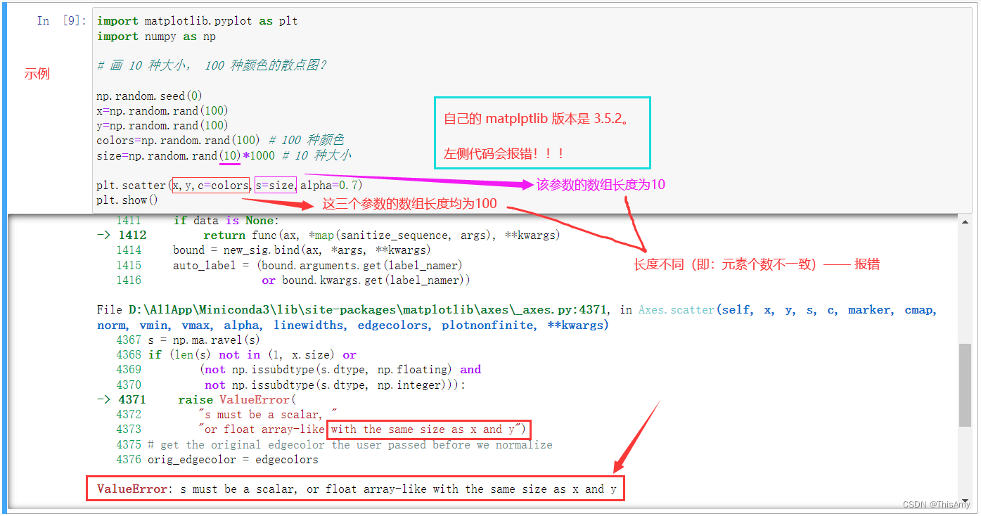
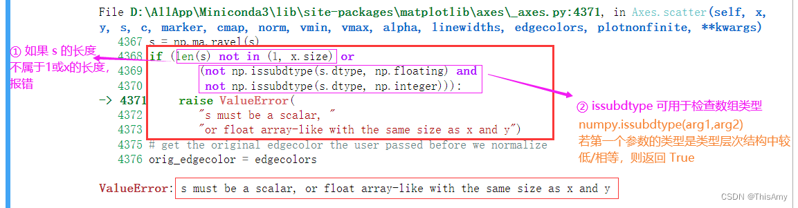
'c' argument has 5110 elements, which is inconsistent with 'x' and 'y' with size 4909.怎么解决?


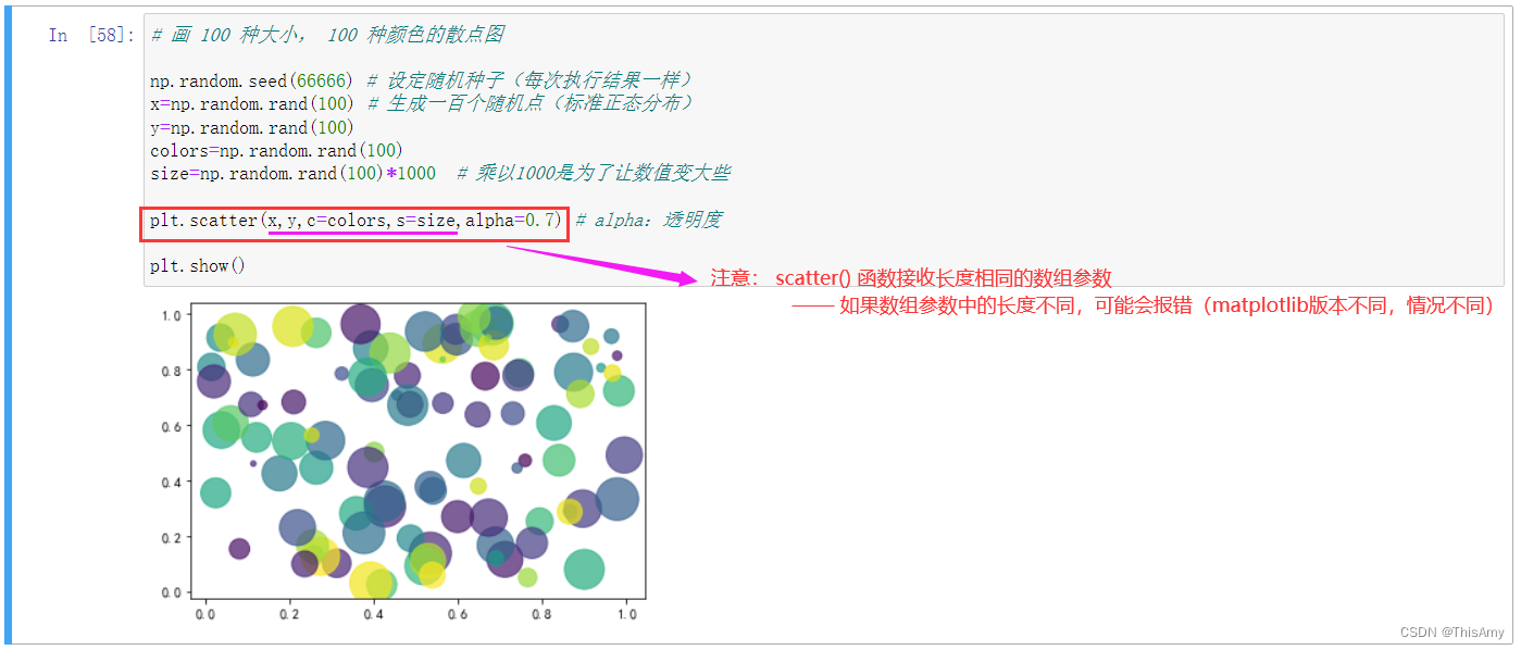
 在Windows的Jupyter Notebook中使用Matplotlib 3.5.2绘制散点图时遇到ValueError。错误提示`s`必须是标量或与`x`和`y`尺寸相同的浮点数数组。问题出在`size`数组长度不匹配。修正代码将`size`数组长度调整为与`x`和`y`相同,即可解决该错误。示例代码展示了如何正确绘制100种大小和颜色的散点图。


 5311
5311

 被折叠的 条评论
为什么被折叠?
被折叠的 条评论
为什么被折叠?
 到【灌水乐园】发言


