


论文原名:Preserving specificity in federated graph learning for fMRI-based neurological disorder identification
论文代码:ZJH123333/SFGL:SFGL 框架的源代码 (github.com)
英文是纯手打的!论文原文的summarizing and paraphrasing。可能会出现难以避免的拼写错误和语法错误,若有发现欢迎评论指正!文章偏向于笔记,谨慎食用
目录
2.3.1. Graph learning for functional MRI analysis
2.3.2. Federated learning for brain disease analysis
2.4. Materials and data preprocessing
2.5.2. Personalized branch at client side
2.5.3. Federated aggregation at server side
2.6.4. Statistical significance analysis
2.7.2. Influence of balancing coefficient
2.7.3. Influence of local training epoch
2.7.5. Influence of feature extractor
2.7.6. Interpretable biomarker analysis
2.7.8. Model scalability analysis
2.7.9. Computation cost analysis
2.7.10. Limitations and future work
1. 省流版
1.1. 心得
(1)怎么讲呢,看开头觉得模型上没什么创新点,联邦学习上的改进也只是加入了一些非图像因素
(2)扫描参数是官方给的吧?意思是直接抄进来了?
(3)每个站点单独的数据还是有点少
2. 论文逐段精读
2.1. Abstract
①Crossing site fMRI analysis faces data privacy, security problems and storage burden
②Previous FL methods in brain disease classification ignored site-specificity
2.2. Introduction
①There are privacy problems/hazard in multi-site imaging data analysis
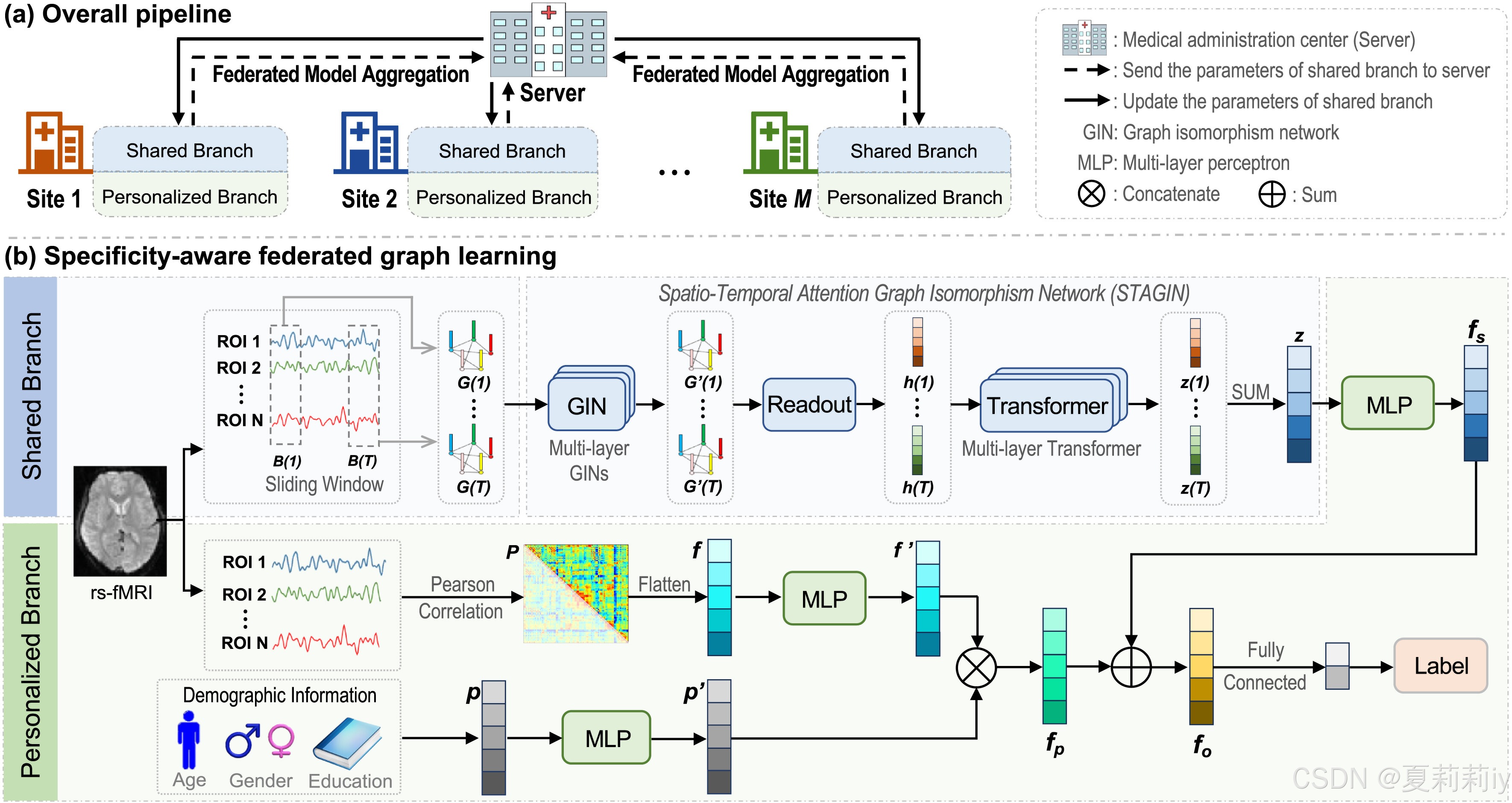
②They proposed a specificity-aware federated graph learning (SFGL) for diagnosing diseases by fMRI:
③Datasets: ABIDE and REST-meta-MDD
2.3. Related work
2.3.1. Graph learning for functional MRI analysis
①Listing spatial and temporal graph methods which applied to mental disease diagnosis
②They further point out the privacy problems
2.3.2. Federated learning for brain disease analysis
①Listing examples of federated learning on brain disease diagnosis
②但作者觉得那些方法没考虑demographic factors (i.e., age, gender, and education)。。。
2.4. Materials and data preprocessing
2.4.1. Materials
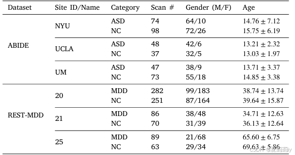
①Demographic data on two datasets:
2.4.2. Data preprocessing
(1)ABIDE I
①Sites: the New York University (NYU), the University of California, Los Angeles (UCLA), and the University of Michigan (UM) (the largest 3)
②Samples: (74+98)+(48+37)+(47+73)=377
③Scanning parameters:
| NYU | 3T Allegra scanner with repetition time (TR) = 2000 ms, echo time (TE) = 15 ms, voxel size = 3.0×3.0×4.0 mm^3, flip angle = 90°, field-of-view (FOV) = 192×240 mm^2 and a total of 33 slices with a thickness of 4 mm. |
| UCLA | 3T Trio scanner with TR = 3000ms, TE = 28 ms, voxel size = 3.0×3.0×4.0 mm^3, flip angle = 90°, FOV = 192×192 mm^2 and a total of 34 slices with a thickness of 4mm. |
| UM | 3T GE Signa scanner with TR = 2000 ms, TE = 30 ms, voxel size = 3.438×3.438×3.000 mm^3, flip angle = 90° and a total of 40 slices with a thickness of 3 mm. |
④Tool: DPARSF
⑤Preprocessing steps: discard the first five volumes, perform head motion correction, spatial smoothing and normalization, bandpass filtering (0.01–0.10 Hz) of BOLD time series, nuisance signals regression, and spatial standardization of the Montreal Neurological Institute (MNI)
⑥Atlas: AAL 116
(2)REST-meta-MDD
①Sites: Site 20, Site 21, and Site 25 (the largest 3)
②Samples: (282+251)+(86+70)+(89+63)=841
③Scanning parameters:
| Site 20 | 3T Trio scanner with a 12-channel receiver coil, with TR = 2000 ms, TE = 30ms, voxel size = 3.44×3.44×4.00mm^ 3, flip angle = 90°, gap = 1.0 mm, FOV = 220×220 mm^2 and a total of 32 slices with a thickness of 3mm |
| Site 21 | 3T Trio scanner with a 32-channel receiver coil, with TR = 2000ms, TE = 30 ms, voxel size = 3.12×3.12×4.20 mm^3, flip angle = 90°, gap = 0.7 mm, FOV = 200×200 mm^2 and a total of 33 slices with a thickness of 3.5 mm |
| Site 25 | 3T Verio scanner with a 12-channel receiver coil, with TR = 2000 ms, TE = 25 ms, voxel size = 3.75×3.75×4.00 mm^3, flip angle = 90°, gap = 0.0 mm, FOV = 240×240 mm^2 and a total of 36 slices with a thickness of 4 mm. |
④Tool: DPARSF
⑤Preprocessing steps: discard the first ten volumes, and employ the same head motion correction, spatial smoothing and normalization, bandpass filtering (0.01–0.10 Hz), nuisance signal regression, and spatial standardization.
⑥Atlas: AAL 116
2.5. Methodology
2.5.1. Shared branch at client side
(1)Dynamic graph sequence construction
①Graph can be noted as where
is the ROI and
reveals the connection set
②BOLD signal: with
ROI and
time points
③They employed slicing window technique. Namely for window length and stride of
, the segment number is
④The BOLD signal in the
-th segment is
⑤The Pearson correlation of the -th ROI and the
-th ROI in the
-th segment can be calculated by
, where
denotes the covatiance and
is standard deviation. Each FCN is denoted by
⑥Node feature matrix:
⑦Sparsify: only retain the top 30% correlation connections in the FCNs and set them as 1:
⑧They construct graph for each time window for each subject:
(2)Dynamic graph representation learning
①They choose STAGIN as the backbone(如果没见过的可以参考:[论文精读]Learning Dynamic Graph Representation of Brain Connectome with Spatio-Temporal Attention-优快云博客)
②Layer of GIN: 2
③SERO(是STAGIN的一个模块)depicted by the authors:

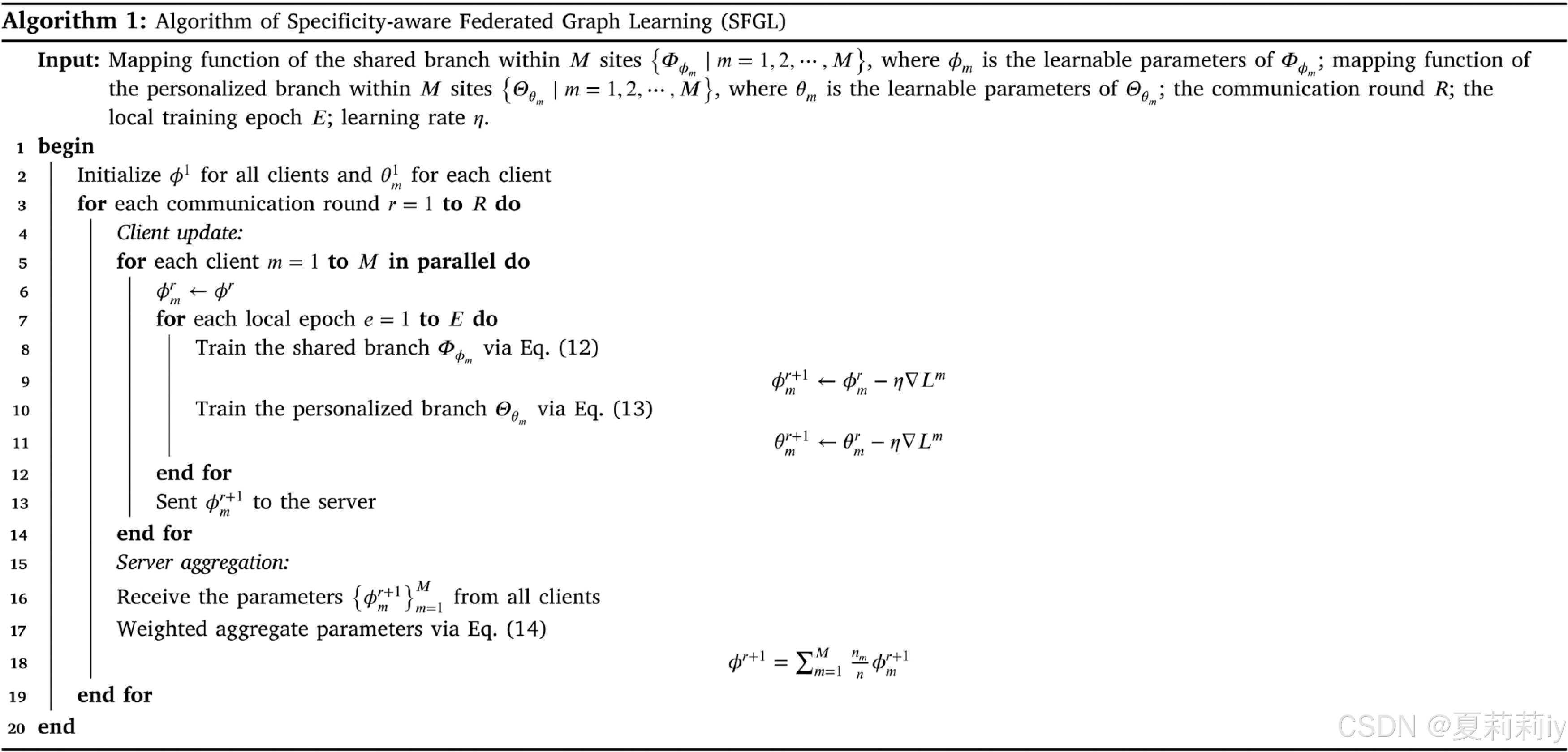
④Pseudo code of SFGL:
2.5.2. Personalized branch at client side
①影像特征:这分支已经非常简单了,使用整个BOLD来求得FC矩阵,然后展平上三角或下三角,再MLP一下。
②非影像特征:把性别年龄和教育串联再一起,再MLP
③Personal feature: concatenate image features and non-image features:
④最后作者把STAGIN得到的和这个personal feature按权重加起来,注意是加起来不是串联了(MLP最后得到的维度一样就能加):
2.5.3. Federated aggregation at server side
①Output of client:
②Output of client further updated by demographic information and imaging features
:
③Cross entropy loss in each branch:
④To prevent the gradient explosion or vanishing, they introduced orthogonal constraint loss:
where
⑤Total loss can be defined as:
⑥Parameter update in client-server communication:
where denotes the learning rate
⑦Parameters in server:
2.5.4. Implementation details
①Batch size: 4
②Dropout rate: 0.5
2.6. Experiments
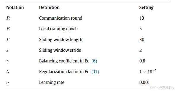
2.6.1. Experimental settings
①Cross validation: 5 fold
②Hyperparameters:
2.6.2. Methods for comparison
①Compared with non-FL and FL strategies respectively.
| non-FL methods | cross method (tr_<site>) | one site for training and others for testing |
| single method | train and test each dataset by 5-fold cross validation separetely | |
| mix | data from all sites are mixed | |
| FL methods | FedAvg | different federated aggregation methods, with mean parameters tranfering |
| FedProx | average server parameters and L2 norm | |
| MOON | maximize the cosine similarity of local and global, minimize the cosine similarity of current communication round and previous | |
| pFedMe | including Moreau envelope | |
| LGFed | only send the parameters in the last fully connected layer |
holistic adj.整体的;全面的;功能整体性的
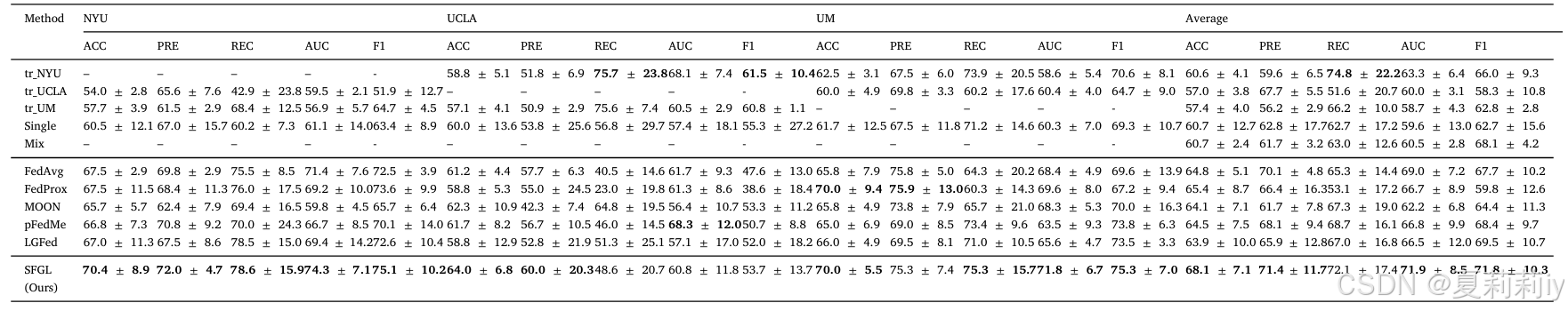
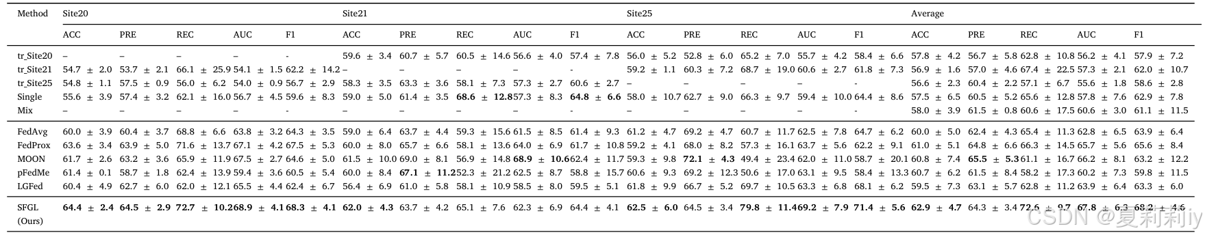
2.6.3. Experimental results
①Comparison table on ABIDE dataset:
②Comparison table on REST-meta-MDD dataset:
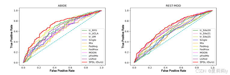
③AUROC curves:
2.6.4. Statistical significance analysis
①Predicted probability distribution between different models:
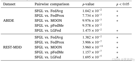
(感觉拿自己模型和别的比也...没什么说服力....)
2.7. Discussion
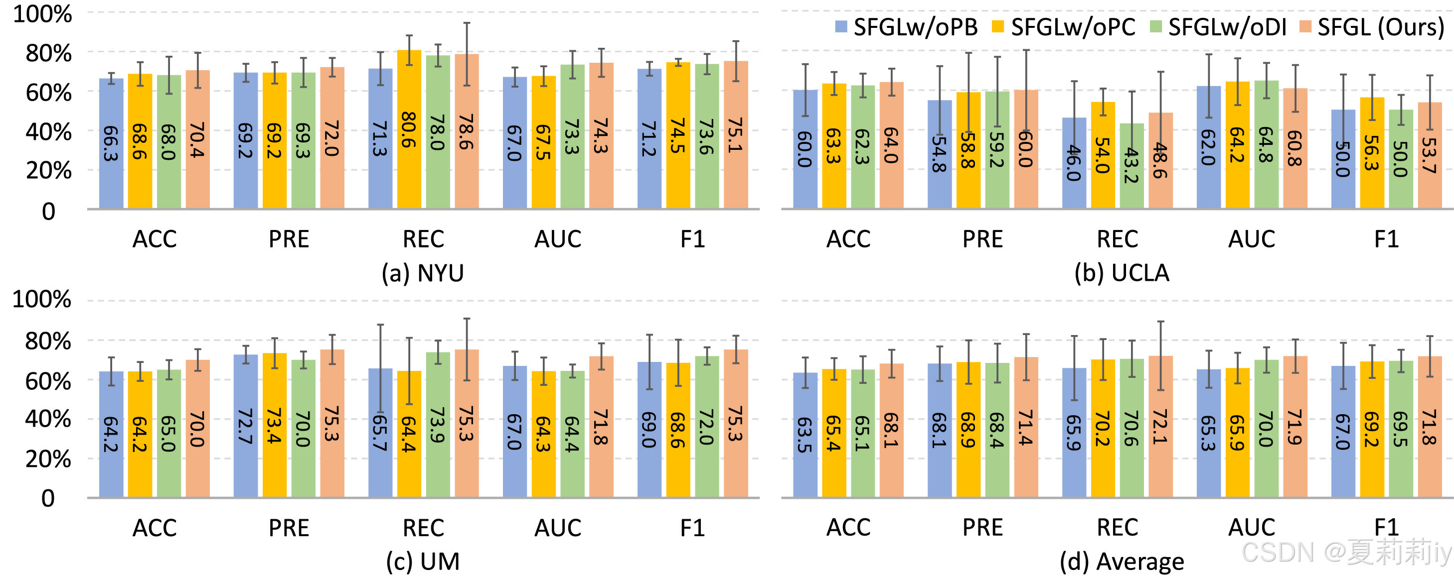
2.7.1. Ablation study
①Considering
| SFGLw/oPB | with shared branch, without personalized branch, sending all local parameters |
| SFGLw/oPC | only using demographic information in personalized branch |
| SFGLw/oDI | only using imaging information in personalized branch |
the ablation study will be:
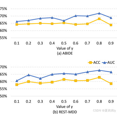
2.7.2. Influence of balancing coefficient
①Grid search on :
2.7.3. Influence of local training epoch
①Grid search of local epoch:
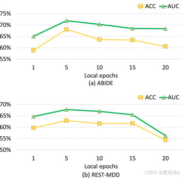
作者觉得epoch太小会频繁更新,大了的话会参数漂移(局部和全局最优的错位)
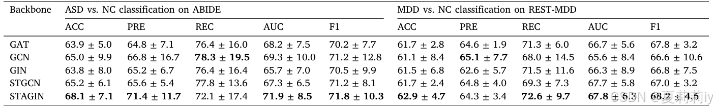
2.7.4. Influence of different backbones in shared branch
①Ablation study with different backbone:
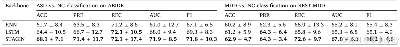
2.7.5. Influence of feature extractor
①Ablation study on different feature extractor:
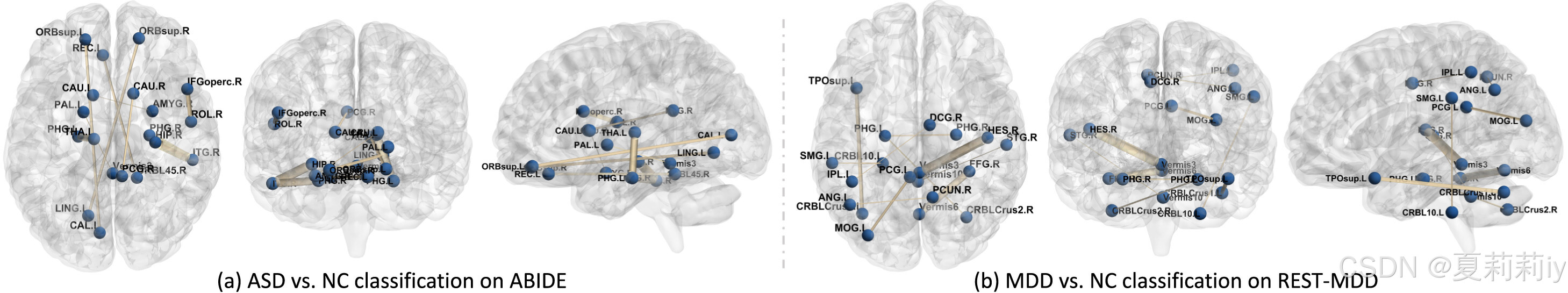
2.7.6. Interpretable biomarker analysis
①Guided back-propagation gradient formula for interpretability:
②The top 10 disctiminative brain regions:
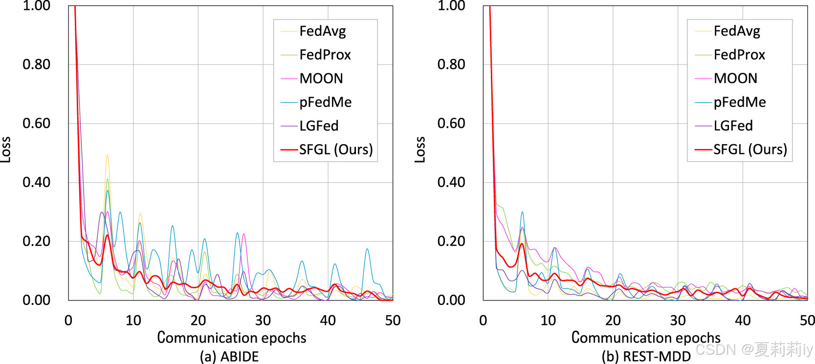
2.7.7. Convergence analysis
①Total number of communication rounds: 10
②Local epoch: 5
③Record of loss:
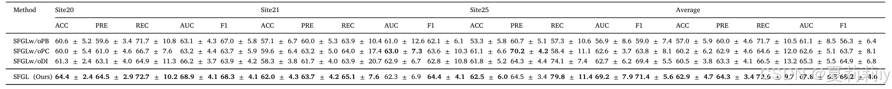
2.7.8. Model scalability analysis
①They adding other sites to identify the scalability of their model:
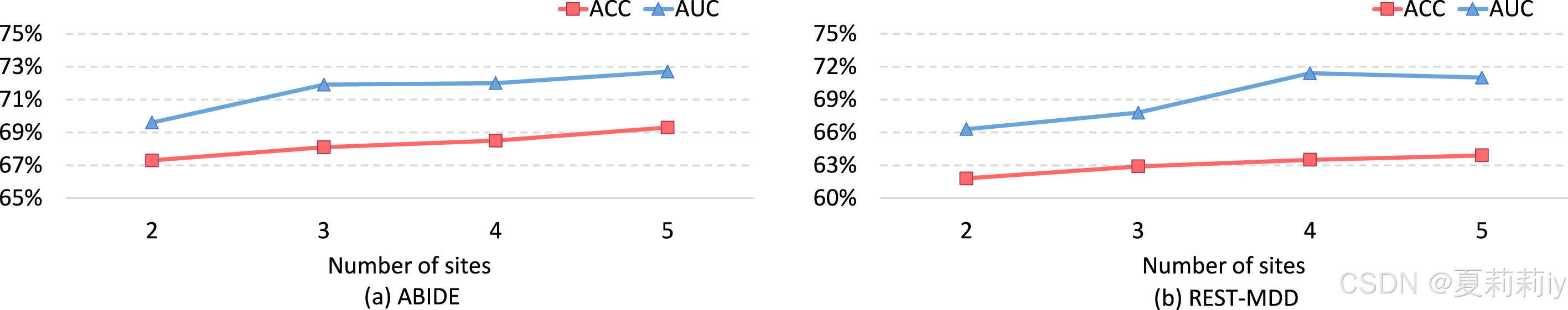
assimilation n.吸收;接受;同化现象;同化
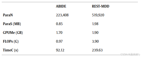
2.7.9. Computation cost analysis
①Computational cost (including the number of model parameters (ParaN), the size of model parameters (ParaS), GPU memory usage during training (GPUMe), floating point operations per second (FLOPs), and the training time for each communication round (TimeC)):
2.7.10. Limitations and future work
①Didn't mention the relationship between subjects
②Personalized branch for each site needed
③More advanced feature fusion strategies required
④Semi-supervised or weak supervised model can be better in the real situation
⑤Weakness in stability and communication efficiency
2.8. Conclusion
Novel in information extraction and federated aggregation approach
4. Reference
Zhang, J. et al. (2024) 'Preserving specificity in federated graph learning for fMRI-based neurological disorder identification', Neural Networks, 169: 584-596. doi: Redirecting


 被折叠的 条评论
为什么被折叠?
被折叠的 条评论
为什么被折叠?
 到【灌水乐园】发言


