【电磁】微带的有限元模拟（Matlab实现）_电磁场有限元开源代码-优快云博客

本文链接：https://blog.youkuaiyun.com/Matlab88888/article/details/143718440

💥💥💞💞 欢迎来到本博客 ❤️❤️💥💥

🏆 博主优势：🌞🌞🌞博客内容尽量做到思维缜密，逻辑清晰，为了方便读者。

⛳️ 座右铭：行百里者，半于九十。

📋📋📋 本文目录如下： 🎁🎁🎁

💥1 概述

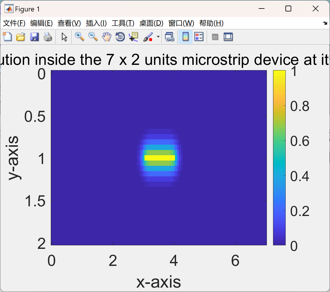
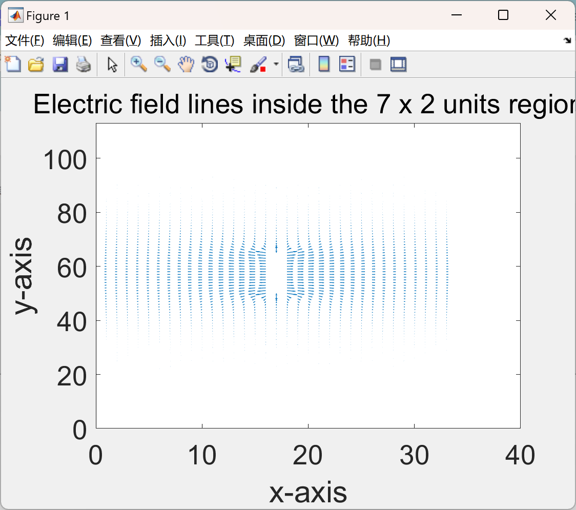
微带的有限元模拟是一种重要的分析方法。微带结构在现代电子技术中有着广泛的应用，如微波电路、天线等领域。有限元模拟通过将微带结构划分成有限个小单元，建立数学模型来近似求解其电磁场分布、传输特性等物理特性。在进行微带的有限元模拟时，首先需要根据微带的几何形状和材料属性建立合适的模型。然后，选择适当的边界条件和求解算法，对模型进行离散化处理。通过求解有限元方程，可以得到微带结构中各个节点处的电场、磁场强度等参数。有限元模拟可以帮助工程师深入了解微带的性能，优化设计参数，提高微带电路和天线的工作效率和可靠性。它可以预测微带的传输损耗、反射系数、辐射特性等，为实际的设计和制造提供重要的参考依据。同时，有限元模拟还可以进行参数化分析，研究不同参数变化对微带性能的影响，从而实现更加高效和精确的设计。

📚2 运行结果

主函数部分代码：

clear all;
clc;

%Dimensions of the simulation grid in x (xdim) and y (ydim) directions
xdim=7;
ydim=2;

%Area of square elements in the grid
area_sq_elem=0.0625^2;

%Step size in the grid in cartesian directions viz. side of the square
%element
step_size=area_sq_elem^0.5;

%No of square elements
sq_elems=(xdim*ydim)/area_sq_elem;

%Dimension in x direction in steps
dim1=xdim/step_size;

%Dimension in y direction in steps
dim2=ydim/step_size;

%No of triangular elements
no_of_elems=sq_elems*2;

%Total no of points for voltage distribution
total_no_pts=(dim1+1)*(dim2+1);

%grid_pts matrix consisting of numbering of all the points in the domain in
%a page read fashion from left to right and then top to bottom along with
%the x and y coordinates of the points in the adjacent columns of the
%matrix
grid_pts=zeros(total_no_pts,3);

%look_up_table matrix consisting of numbering of all the triangular
%elements in a page read fashion just like before along with the cardinal
%numbers of the three points making the triangular elements (obtained from
%the grid_pts matrix) in the adjacent columns of the matrix
look_up_table=zeros(no_of_elems,4);

%Populating the first columns of the above two matrices with serial numbers
i1=1:1:no_of_elems;
look_up_table(:,1)=i1';
i1=1:1:total_no_pts;
grid_pts(:,1)=i1';



% Polpulating the x coordinate and y coordinate columns of the grid_pts
% matrix with the appropriate values from the knowledge of the grid
% geometry
for i1=1:1:total_no_pts
    if rem(i1,dim1+1)==0
        grid_pts(i1,3)=((i1/(dim1+1))-1)*step_size;
    else
        grid_pts(i1,3)=(floor(i1/(dim1+1)))*step_size;
    end
    if rem(i1,dim1+1)==0
        grid_pts(i1,2)=dim1*step_size;
    else
        grid_pts(i1,2)=(i1-(dim1+1)*floor(i1/(dim1+1))-1)*step_size;
    end
end


% Polpulating the second, third and fourth columns of the look_up_table 
% matrix with cardinal numbers (obtained from the grid_pts matrix) of three 
% points forming the corresponding triangular element in the first column.
for i1=1:1:no_of_elems
    k=ceil(i1/(2*dim1))-1;
    if rem(i1,2)==1
        look_up_table(i1,2)=(i1+1)/2+dim1+1+k;
        look_up_table(i1,3)=(i1+1)/2+k;
        look_up_table(i1,4)=(i1+1)/2+1+k;
    else
        look_up_table(i1,2)=i1/2+dim1+1+k;
        look_up_table(i1,3)=i1/2+1+k;
        look_up_table(i1,4)=i1/2+dim1+2+k;
    end
end
        
% Area of all triangular elements are equal to half the area of all square
% elements as they are obtained by dividing the square elements by 2.
area_of_elem=area_sq_elem/2;

% Initializing and populating the P and Q matrices. P and Q matrices are 
% defined for every element as P=(y2-y3,y3-y1,y1-y2) & Q=(x3-x2,x1-x3,x2-x1)
% where (x1,y1),(2,y2),(x3,y3) are the coordinates of the three points
% making up the triangular element starting from the bottom left point and
% moving anti-clockwise. Also, C matrices are iitialized for local eleements
% which is then accumulated into a global matrix
P=zeros(no_of_elems,3);
Q=zeros(no_of_elems,3);
C=zeros(no_of_elems,3,3);
for i1=1:1:no_of_elems
    P(i1,1)=grid_pts(look_up_table(i1,3),3)-grid_pts(look_up_table(i1,4),3);
    P(i1,2)=grid_pts(look_up_table(i1,4),3)-grid_pts(look_up_table(i1,2),3);
    P(i1,3)=grid_pts(look_up_table(i1,2),3)-grid_pts(look_up_table(i1,3),3);
    Q(i1,1)=grid_pts(look_up_table(i1,4),2)-grid_pts(look_up_table(i1,3),2);
    Q(i1,2)=grid_pts(look_up_table(i1,2),2)-grid_pts(look_up_table(i1,4),2);
    Q(i1,3)=grid_pts(look_up_table(i1,3),2)-grid_pts(look_up_table(i1,2),2);
    for j=1:1:3
        for k=1:1:3
            C(i1,j,k)=(1/(4*area_of_elem))*(P(i1,j)*P(i1,k)+Q(i1,j)*Q(i1,k));
        end
    end
end

% Initializing matrix C_global from which propagation voltage distribution 
% is calculated using iterative analysis
C_global=zeros(total_no_pts,total_no_pts);

% Calculating matrix C1_global by adding up local C matrices
for i=1:1:no_of_elems
    for j=1:1:3
        for k=1:1:3
            C_global(look_up_table(i,j+1),look_up_table(i,k+1))=C_global(look_up_table(i,j+1),look_up_table(i,k+1))+C(i,j,k);
        end
    end
end

%Initializing previous (V_prev) voltage distribution matrix viz the voltage
%distribution matrix before any iteration
V_prev=zeros(dim1+1,dim2+1);

% Giving Dirichlet boundary cnditions for previous voltage distribution matrix
% at the plates and microstrip line
V_prev(1,1:dim2+1)=0;
V_prev(dim1+1,1:dim2+1)=0;
V_prev(1:dim1+1,1)=0;
V_prev(1:dim1+1,dim2+1)=0;
V_prev(3*(dim1/7)+2:4*(dim1/7)+1,(dim2/2)+1)=1;%Microstrip line

%Initializing present (V_now) voltage distribution matrix viz the voltage
%distribution matrix after any iteration and the matrix is given a critical
%difference from V_prev matrix at (2,2) to enter loop of update.
V_now=V_prev;
V_now(2,2)=1;

%Iteration counter iter initialized
iter=0;

%Update loop begins with condition as difference between two matrics being
%greater than 0.001
while(max(max(abs(V_prev-V_now)))>1e-3)

    %Iteration counter incremented
    iter=iter+1;
    
    %Initial critical difference between matrices removed in first
    %iteration
    if iter==1
        V_now(2,2)=0;
    end
    
    %Updating V_prev of present iteration with V_now of previous iteration 
    V_prev=V_now;
    %Clearing V_now for update
    V_now(:,:)=0;
    
    %Updating V_now using standard update procedure obtained from FEM
    %analysis
    for k1=1:1:dim2+1
        for k2=1:1:dim1+1
            for i1=1:1:dim2+1
                for i2=1:1:dim1+1
                    if(C_global((k1-1)*(dim1+1)+k2,(i1-1)*(dim1+1)+i2)>0 || C_global((k1-1)*(dim1+1)+k2,(i1-1)*(dim1+1)+i2)<0)
                        if(i1<k1 || i2<k2 || i1>k1 || i2>k2)
                            V_now(k2,k1)=V_now(k2,k1)-(1/C_global((k1-1)*(dim1+1)+k2,(k1-1)*(dim1+1)+k2))*V_prev(i2,i1)*C_global((k1-1)*(dim1+1)+k2,(i1-1)*(dim1+1)+i2);
                        end
                    end
                end
            end
        end
    end
    
    % Giving Dirichlet boundary cnditions for previous voltage distribution matrix
    % at the plates and microstrip line
    V_now(1,1:dim2+1)=0;
    V_now(dim1+1,1:dim2+1)=0;
    V_now(1:dim1+1,1)=0;
    V_now(1:dim1+1,dim2+1)=0;
    V_now(3*(dim1/7)+2:4*(dim1/7)+1,(dim2/2)+1)=1;%Microstrip line