【控制】采用 FxLMS 算法的有源噪声控制系统（Matlab实现）

原创已于 2024-11-09 15:20:35 修改 · 312 阅读

9 ·

CC 4.0 BY-SA版权

文章标签：

#算法

于 2024-11-09 14:57:56 首次发布

💥💥💞💞欢迎来到本博客❤️❤️💥💥

🏆博主优势：🌞🌞🌞博客内容尽量做到思维缜密，逻辑清晰，为了方便读者。

⛳️座右铭：行百里者，半于九十。

📋📋📋本文目录如下：🎁🎁🎁

💥1 概述

采用 FxLMS 算法的有源噪声控制系统是一种先进的噪声控制技术。该系统的核心是 FxLMS（Filtered-x Least Mean Square）算法。这一算法通过对输入的噪声信号进行分析和处理，以实现有效的噪声消除。有源噪声控制系统通常由传感器、控制器和执行器组成。传感器用于检测噪声信号，将其转换为电信号输入到控制器中。控制器利用 FxLMS 算法对输入信号进行计算和处理，生成控制信号。执行器则根据控制信号产生与噪声相反的声波，从而实现对噪声的抵消。 FxLMS 算法具有自适应能力，能够根据噪声环境的变化实时调整控制参数，以保持良好的噪声控制效果。它可以处理各种类型的噪声，包括稳态噪声、非稳态噪声和随机噪声等。这种有源噪声控制系统在许多领域具有广泛的应用前景。例如，在工业环境中，可以降低机器设备产生的噪声，提高工作环境的舒适度和安全性；在交通运输领域，可以减少车辆、飞机等交通工具的噪声，提升乘坐体验；在音频设备中，可以改善音质，降低背景噪声的干扰。总之，采用 FxLMS 算法的有源噪声控制系统是一种高效、灵活的噪声控制解决方案，为改善噪声环境提供了有力的技术支持。

📚2 运行结果

主函数部分代码：

clear
T=1000; 

% We do not know P(z) and S(z) in reality. So we have to make dummy paths
Pw=[0.01 0.25 0.5 1 0.5 0.25 0.01];
Sw=Pw*0.25;

% Remember that the first task is to estimate S(z). So, we can generate a
% white noise signal,
x_iden=randn(1,T);

% send it to the actuator, and measure it at the sensor position, 
y_iden=filter(Sw, 1, x_iden);

% Then, start the identification process
Shx=zeros(1,16);     % the state of Sh(z)
Shw=zeros(1,16);     % the weight of Sh(z)
e_iden=zeros(1,T);   % data buffer for the identification error

% and apply least mean square algorithm
mu=0.1;                         % learning rate
for k=1:T,                      % discrete time k
    Shx=[x_iden(k) Shx(1:15)];  % update the state
    Shy=sum(Shx.*Shw);	        % calculate output of Sh(z)
    e_iden(k)=y_iden(k)-Shy;    % calculate error         
    Shw=Shw+mu*e_iden(k)*Shx;   % adjust the weight
end

% Lets check the result
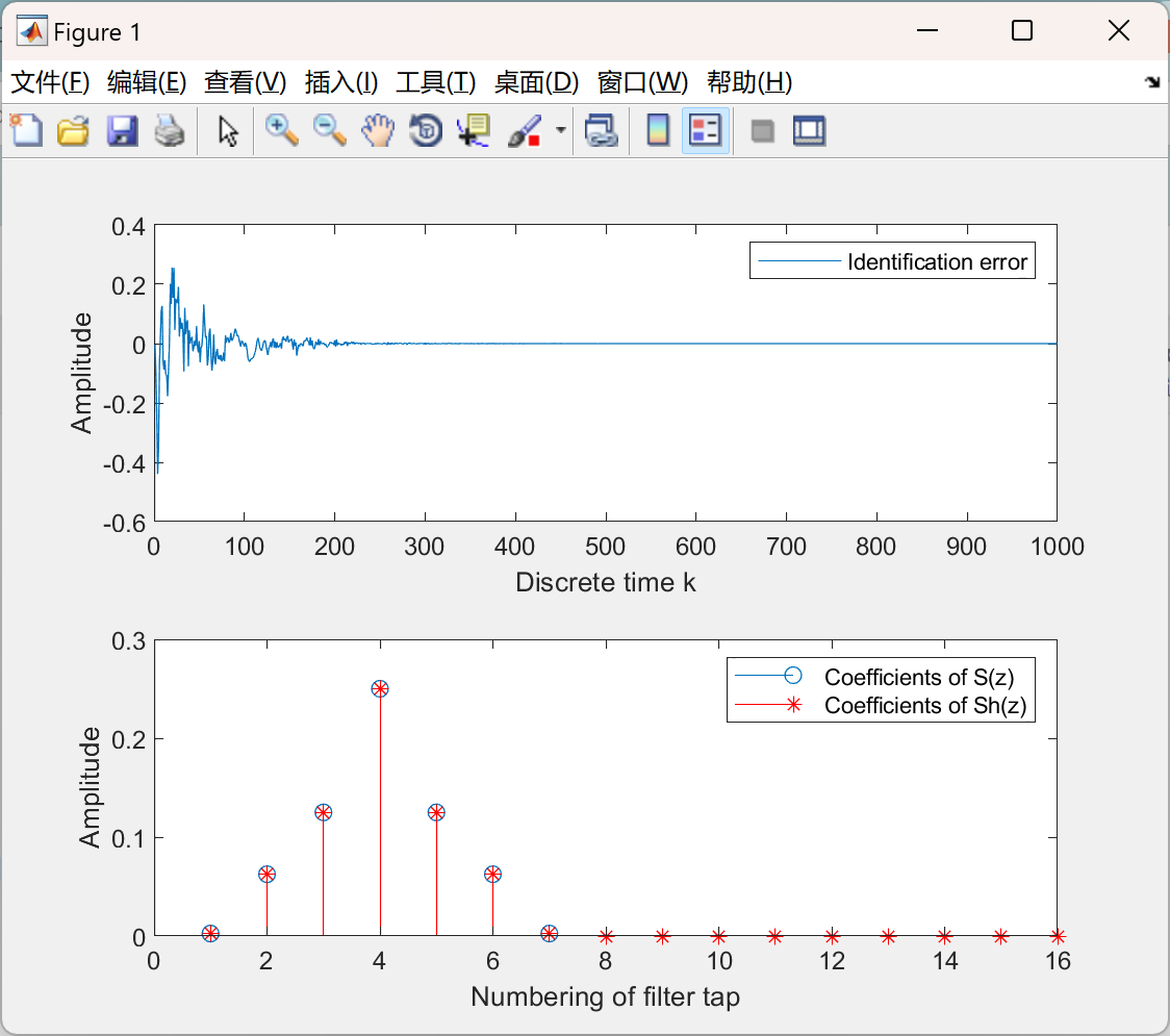
subplot(2,1,1)
plot([1:T], e_iden)
ylabel('Amplitude');
xlabel('Discrete time k');
legend('Identification error');
subplot(2,1,2)
stem(Sw) 
hold on 
stem(Shw, 'r*')
ylabel('Amplitude');
xlabel('Numbering of filter tap');
legend('Coefficients of S(z)', 'Coefficients of Sh(z)')


% The second task is the active control itself. Again, we need to simulate 
% the actual condition. In practice, it should be an iterative process of
% 'measure', 'control', and 'adjust'; sample by sample. Now, let's generate 
% the noise: 
X=randn(1,T);

% and measure the arriving noise at the sensor position,
Yd=filter(Pw, 1, X);
  
% Initiate the system,
Cx=zeros(1,16);       % the state of C(z)
Cw=zeros(1,16);       % the weight of C(z)
Sx=zeros(size(Sw));   % the dummy state for the secondary path
e_cont=zeros(1,T);    % data buffer for the control error
Xhx=zeros(1,16);      % the state of the filtered x(k)

% and apply the FxLMS algorithm
mu=0.1;                            % learning rate
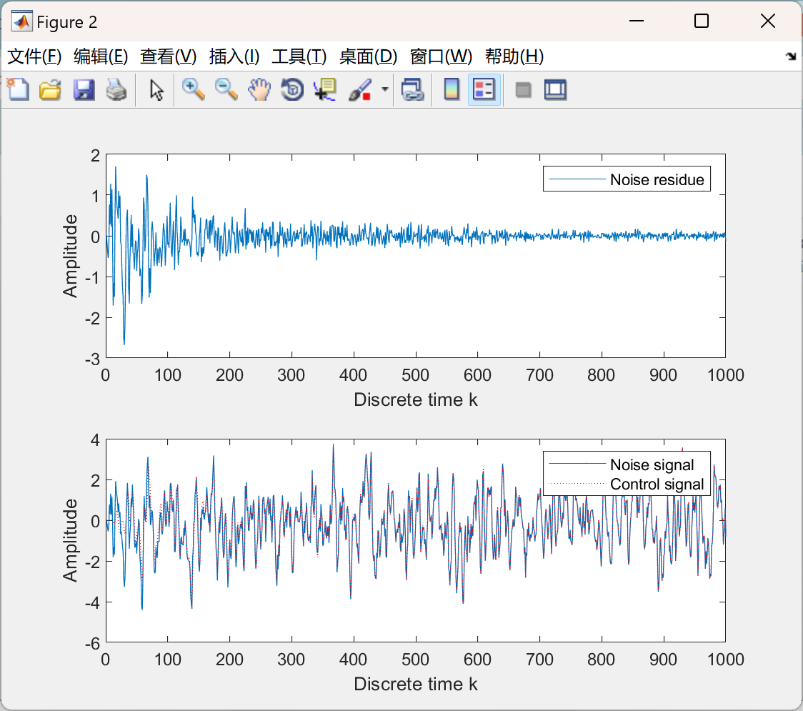
for k=1:T,                         % discrete time k
    Cx=[X(k) Cx(1:15)];            % update the controller state    
    Cy=sum(Cx.*Cw);                % calculate the controller output	
    Sx=[Cy Sx(1:length(Sx)-1)];    % propagate to secondary path
    e_cont(k)=Yd(k)-sum(Sx.*Sw);   % measure the residue
    Shx=[X(k) Shx(1:15)];          % update the state of Sh(z)
    Xhx=[sum(Shx.*Shw) Xhx(1:15)]; % calculate the filtered x(k)
    Cw=Cw+mu*e_cont(k)*Xhx;        % adjust the controller weight
end