【MPC】使用输入增量实现了不同的状态空间MPC公式研究（Matlab代码实现）

 💥💥💞💞欢迎来到本博客❤️❤️💥💥

🏆博主优势：🌞🌞🌞博客内容尽量做到思维缜密，逻辑清晰，为了方便读者。

⛳️座右铭：行百里者，半于九十。

📋📋📋本文目录如下：🎁🎁🎁

目录

💥1 概述

📚2 运行结果

🎉3 参考文献

🌈4 Matlab代码实现

---

💥1 概述

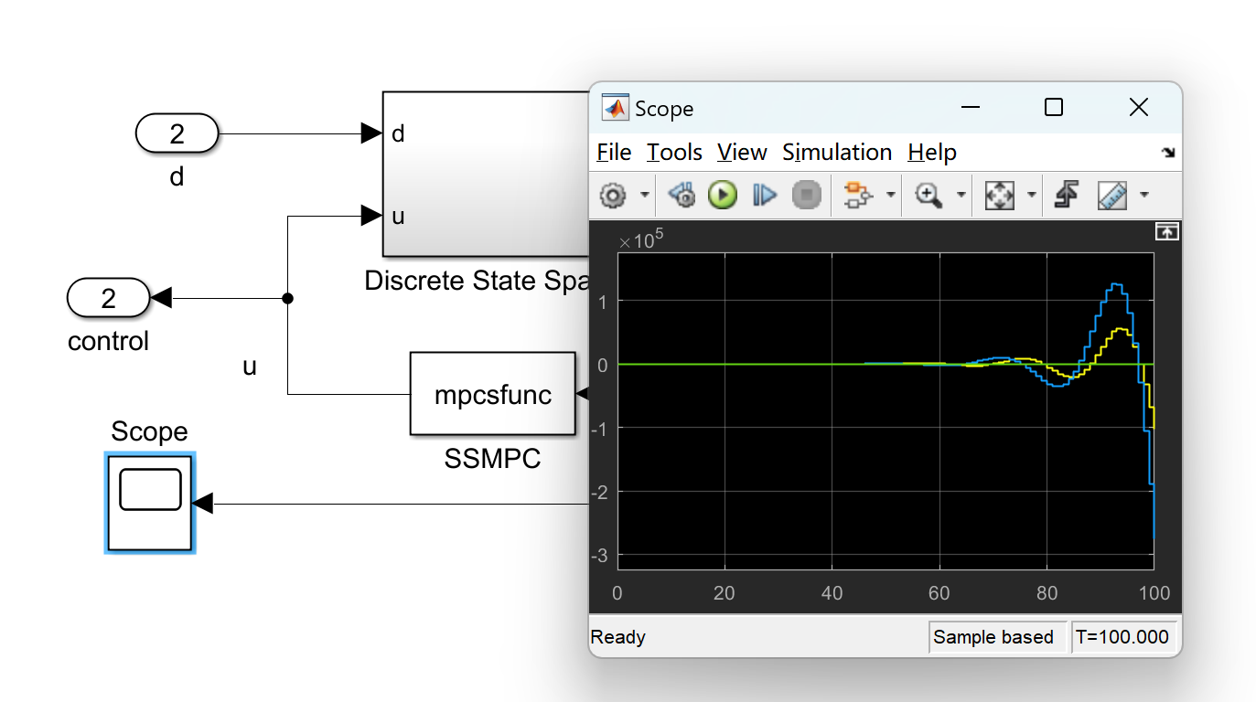
在本MPC教程中，我们将重点介绍如何使用输入增量的状态空间MPC来实现控制系统。我们将通过函数和simulink块来展示如何在状态空间MPC中使用输入增量。通过本文的学习，您将了解到如何利用输入增量实现不同的状态空间MPC公式，并且能够在m-function和simulink中进行实现。

使用输入增量的状态空间MPC公式在避免了逆矩阵的计算的同时，也提高了其通用性。这意味着无论是在理论研究还是实际应用中，都能够更加灵活地应用这种方法。通过本教程，您将掌握如何利用输入增量的状态空间MPC来实现更加高效和通用的控制系统，为您的工程项目带来更多的可能性和灵活性。

📚2 运行结果

部分代码：
 

%% Simulation
% 150 seconds (1500 sampling intervals) simulation is conducted with
% several setpoint changes and random cooling water temperature changes
% within positive and negative 1 degree.
% Simulation length and variables for results
N=1500;
x0=zeros(6,1);
Y=zeros(N,2);
U=zeros(N,2);
% Predefined reference
T=zeros(N,2);
T(10:N,1)=1;
T(351:N,1)=3;
T(600:N,1)=5;
T(1100:N,1)=3;
T(100:N,2)=2;
T(451:N,2)=1;
T(700:N,2)=4;
T(1200:N,2)=2;
% Simulation
%%
for k=1:N
    % Process disturbances
    w=Bd*(rand(2,1)-0.5)*2;
    % Measurements noise
    v=0.01*randn(2,1);
    % actual measurement
    y=C*x0+v;
    % online controller
    u=ssmpc(y,T(k:end,:)');
    % plant update
    x0=A*x0+Bu*u+w;
    % save results
    Y(k,:)=y';
    U(k,:)=u';
end

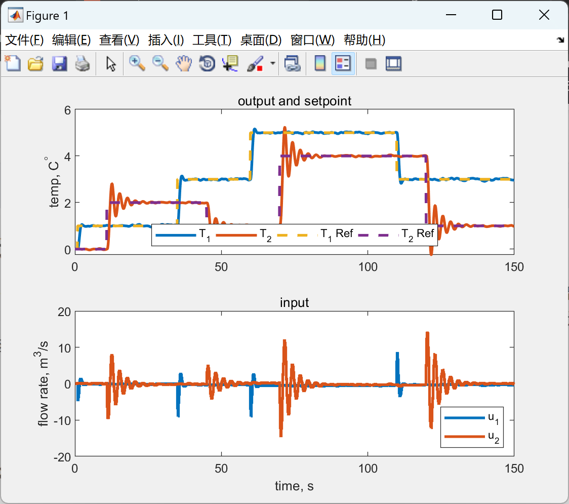
%% Results
% The simulation results are summarized in two sub-plots.
t=(0:N-1)*0.1;
subplot(211)
plot(t,Y,t,T,'--','linewidth',2)
title('output and setpoint')
ylabel('temp, C^\circ')
legend('T_1','T_2','T_1 Ref','T_2 Ref','location','south','Orientation','horizontal')
subplot(212)
stairs(t,U,'linewidth',2)
legend('u_1','u_2','location','southeast')
title('input')
ylabel('flow rate, m^3/s')
xlabel('time, s')

🎉3 参考文献

文章中一些内容引自网络，会注明出处或引用为参考文献，难免有未尽之处，如有不妥，请随时联系删除。

[1]周锐森,冯友兵.基于状态空间MPC的无人机无人车联合运动控制[J].计算机与数字工程, 2021, 049(011):2383-2390.

[2]周锐森,冯友兵.基于状态空间MPC的无人机无人车联合运动控制[J].计算机与数字工程, 2021, 49(11):8.

🌈4 Matlab代码实现