cp4 TrainingSetsPreprocessing_2_ Sequential feature selection_vs_Rand_tree_combinations_knn_format_%

本文链接：https://blog.youkuaiyun.com/Linli522362242/article/details/108272169

本文探讨了特征选择的重要性，介绍了L1正则化避免过拟合的方法，以及使用顺序特征选择算法进行特征子集优化的过程。通过实例展示了特征减少对模型性能的影响，并讨论了随机森林在特征重要性评估中的应用。

摘要生成于 C知道，由 DeepSeek-R1 满血版支持，前往体验 >

cp4 Training Sets Preprocessing_StringIO_dropna_categorical_feature_Encode_Scale_L1_L2_bbox_to_anchor: https://blog.youkuaiyun.com/Linli522362242/article/details/108230328

Sequential feature selection algorithms

An alternative way to reduce the complexity of the model and avoid overfitting is dimensionality reduction via feature selection, which is especially useful for unregularized models. There are two main categories of dimensionality reduction techniques: feature selection and feature extraction. Using feature selection, we select a subset of the original features. In feature extraction, we derive information from the feature set to construct a new feature subspace. In this section, we will take a look at a classic family of feature selection algorithms. In the next chapter, Chapter 5, Compressing Data via Dimensionality Reduction, we will learn about different feature extraction techniques to compress a dataset onto a lower dimensional feature subspace.
cp5_Compressing Data via Dimensionality Reduction_feature extraction_PCA_LDA_convergence_kernel PCA:https://blog.youkuaiyun.com/Linli522362242/article/details/105196037

In this section, we will take a look at a classic family of feature selection algorithms. In the next chapter, Chapter 5, Compressing Data via Dimensionality Reduction, we will learn about different feature extraction techniques to compress a dataset onto a lower-dimensional feature subspace.

Sequential feature selection (for supervised learning) algorithms are a family of greedy search algorithms that are used to reduce an initial d-dimensional feature space to a k-dimensional feature subspace where k<d. The motivation behind feature selection algorithms is to automatically select a subset of features that are most relevant to the problem, to improve computational efficiency or reduce the generalization error of the model by removing irrelevant features or noise, which can be useful for algorithms that don't support regularization.

A classic sequential feature selection algorithm is Sequential Backward Selection (SBS), which aims to reduce the dimensionality of the initial feature subspace with a minimum decay最小衰减 in performance of the classifier to improve upon computational efficiency. In certain cases, SBS can even improve the predictive power of the model if a model suffers from overfitting.

################################################################

Note
Greedy algorithms make locally optimal choices at each stage of a combinatorial search problem and generally yield a suboptimal solution to the problem, in contrast to exhaustive search algorithms, which evaluate all possible combinations and are guaranteed to find the optimal solution. However, in practice, an exhaustive search is often computationally not feasible, whereas greedy algorithms allow for a less complex, computationally more efficient solution.

################################################################

The idea behind the SBS algorithm is quite simple: SBS sequentially removes features from the full feature subset until the new feature subspace contains the desired number of features. In order to determine which feature is to be removed at each stage, we need to define the criterion function J that we want to minimize. The criterion calculated by the criterion function can simply be the difference in performance of the classifier before and after the removal of a particular feature. Then, the feature to be removed at each stage can simply be defined as the feature that maximizes this criterion; or in more intuitive terms, at each stage we eliminate the feature that causes the least performance loss after removal. Based on the preceding definition of SBS, we can outline the algorithm in four simple steps:

1. Initialize the algorithm with k=d, where d is the dimensionality of the full feature space .
2. Determine the feature that maximizes the criterion: , where .
3. Remove the feature from the feature set: .
4. Terminate if k equals the number of desired features; otherwise, go to step 2.

############################################################

Note
You can find a detailed evaluation of several sequential feature algorithms in Comparative Study of Techniques for Large-Scale Feature Selection, F. Ferri, P. Pudil, M. Hatef, and J. Kittler, pages 403-413, 1994.

############################################################

Unfortunately, the SBS algorithm has not been implemented in scikit-learn yet. But since it is so simple, let us go ahead and implement it in Python from scratch:

from sklearn.base import clone
from itertools import combinations
import numpy as np
from sklearn.metrics import accuracy_score
from sklearn.model_selection import train_test_split

class SBS():
    def __init__(self, estimator, k_features, scoring=accuracy_score, test_size=0.25, random_state=1):
        self.scoring = scoring #criterion 
        self.estimator = clone(estimator)
        self.k_features = k_features
        self.test_size = test_size
        self.random_state = random_state
        
    def _calc_score(self, X_train, y_train, X_test, y_test, indices):
        self.estimator.fit(X_train[:, indices], y_train)
        y_pred = self.estimator.predict(X_test[:, indices])#indices: indices of selected features
        score = self.scoring(y_test, y_pred) #criterion, e.g. Return the mean accuracy on the given test data and labels.
        return score
    
    def fit(self, X,y):
        X_train, X_test, y_train, y_test = train_test_split(X,y, 
                                                            test_size=self.test_size, 
                                                            random_state=self.random_state)
        
        dim = X_train.shape[1] #features  # Initialize the algorithm with k=d, d full features
        self.indices_ = tuple(range(dim)) # indices of all features
        self.subsets_ = [self.indices_]
        score = self._calc_score(X_train, y_train,
                                 X_test, y_test, self.indices_)# for all features
        self.scores_ = [score]
        
        while dim > self.k_features:
            temp_scores = []
            subsets = []
            
            #len(p) = r, and p is a subset of self.indices_
            for p in combinations(self.indices_, r=dim-1):
                score = self._calc_score(X_train, y_train,
                                         X_test, y_test, p)
                temp_scores.append(score)
                subsets.append(p)
            # Determine the feature x`(will be removed) that maximizes the criterion    
            bestFeaturesComb = np.argmax(temp_scores)
            self.indices_ = subsets[bestFeaturesComb] # select features without x`
            self.subsets_.append(self.indices_)    ####### feature subsets
            dim -=  1
            
            self.scores_.append(temp_scores[bestFeaturesComb]) ####### until len(bestFeaturesComb)==k
        self.k_score_ = self.scores_[-1]
        
        return self
    
    def transform(self, X):
        return X[:, self.indices_] #self_indices <== len(bestFeaturesComb)==k

In the preceding implementation, we defined the k_features parameter to specify the desired number of features we want to return. By default, we use the accuracy_score from scikit-learn to evaluate the performance of a model (an estimator for classification) on the feature subsets. Inside the while loop of the fit method, the feature subsets created by the itertools.combinations function are evaluated and reduced until the feature subset has the desired dimensionality. In each iteration, the accuracy score of the best subset is collected in a list, self.scores_, based on the internally created test dataset X_test. We will use those scores later to evaluate the results. The column indices of the final feature subset are assigned to self.indices_, which we can use via the transform method to return a new data array with the selected feature columns. Note that, instead of calculating the criterion explicitly inside the fit method, we simply removed the feature that is not contained in the best performing feature subset.

Now, let us see our SBS implementation in action using the KNN classifier from scikit-learn:

import matplotlib.pyplot as plt
from sklearn.neighbors import KNeighborsClassifier

knn = KNeighborsClassifier(n_neighbors=5)

# selecting features
sbs = SBS(knn, k_features=1)
sbs.fit(X_train_std, y_train)

Although our SBS implementation already splits the dataset into a test and training dataset inside the fit function, we still fed the training dataset X_train to the algorithm. The SBS fit method will then create new training subsets for testing (validation) and training, which is why this test set is also called the validation dataset. This approach is necessary to prevent our original test set from becoming part of the training data.

knn.get_params()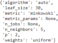

# The default metric is minkowski, and with p=2 is equivalent to the standard Euclidean metric.
It becomes the Euclidean distance if we set the parameter p=2 or the Manhattan distance at p=1. https://blog.youkuaiyun.com/Linli522362242/article/details/107843678

Remember that our SBS algorithm collects the scores of the best feature subset at each stage, so let us move on to the more exciting part of our implementation and plot the classification accuracy of the KNN classifier that was calculated on the
validation dataset. The code is as follows:

# plotting performance of feature subsets
k_feat = [len(k) for k in sbs.subsets_] # len(k) is from X_train.shape[1] to k_features

plt.plot(k_feat, sbs.scores_, marker='o')
plt.ylim([0.7, 1.02])
plt.ylabel("Accuracy")
plt.xlabel("Number of features")
plt.grid()
plt.tight_layout()
plt.show()

As we can see in the following figure, the accuracy of the KNN classifier improved on the validation dataset as we reduced the number of features, which is likely due to a decrease in the curse of dimensionality that we discussed in the context of the KNN algorithm in Chapter 3, A Tour of Machine Learning Classifiers Using scikitlearn. Also, we can see in the following plot that the classifier achieved 100 percent accuracy for k={3, 7, 8, 9, 10, 11, 12}:

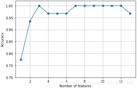
To satisfy our own curiosity, let's see what the smallest feature subset (k=3) that yielded such a good performance on the validation dataset looks like:

k3 = list(sbs.subsets_[10]) # X_train.shape[1]== 13-10=3
print(df_wine.columns[1:][k3])

Using the preceding code, we obtained the column indices of the three-feature subset from the 10th position in the sbs.subsets_ attribute and returned the corresponding feature names from the column-index of the pandas Wine DataFrame.

Next let's evaluate the performance of the KNN classifier on the original test set:

knn.fit(X_train_std, y_train)
print('Training accuracy:', knn.score(X_train_std, y_train))

print('Test accuracy:', knn.score(X_test_std, y_test))

In the preceding code section, we used the complete feature set and obtained approximately 97 percent accuracy on the training dataset and approximately 96 percent accuracy on the test, which indicates that our model already generalizes well to new data.

Now, let us use the selected three-feature subset and see how well KNN performs:

knn.fit(X_train_std[:,k3], y_train)
print('Training accuracy:', knn.score(X_train_std[:,k3], y_train))

print('Test accuracy:', knn.score(X_test_std[:,k3], y_test))

Using less than a quarter of the original features in the Wine dataset, the prediction accuracy on the test set declined slightly. This may indicate that those three features do not provide less discriminatory information than the original dataset. However, we also have to keep in mind that the Wine dataset is a small dataset, which is very susceptible to randomness—that is, the way we split the dataset into training and test subsets, and how we split the training dataset further into a training and validation subset.

While we did not increase the performance of the KNN model by reducing the number of features, we shrank the size of the dataset, which can be useful in realworld applications that may involve expensive data collection steps. Also, by substantially reducing the number of features, we obtain simpler models, which are easier to interpret.

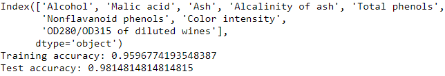
k8 = list(sbs.subsets_[5])
knn.fit(X_train_std[:,k8], y_train)
print(df_wine.columns[1:][k8])
print('Training accuracy:', knn.score(X_train_std[:,k8], y_train))
print('Test accuracy:', knn.score(X_test_std[:,k8], y_test))

Using fewer than half of the original features in the Wine dataset, the prediction accuracy on the test set improved by almost 2 percent (vs test accuracy). Also, we reduced overfitting, which we can tell from the small gap between test (~98 percent) and training (~96.0 percent) accuracy.

####################################################

Note
Feature selection algorithms in scikit-learn

There are many more feature selection algorithms available via scikit-learn. Those include recursive backward elimination based on feature weights, tree-based methods to select features by importance, and univariate statistical tests. A comprehensive discussion of the different feature selection methods is beyond the scope of this book, but a good summary with illustrative examples can be found at http://scikit-learn.org/stable/modules/feature_selection.html. Furthermore, I implemented several different flavors of sequential feature selection, related to the simple SBS that we implemented previously. You can find these implementations in the Python package mlxtend at http://rasbt.github.io/mlxtend/user_guide/feature_selection/SequentialFeatureSelector/

https://blog.youkuaiyun.com/Linli522362242/article/details/104542381

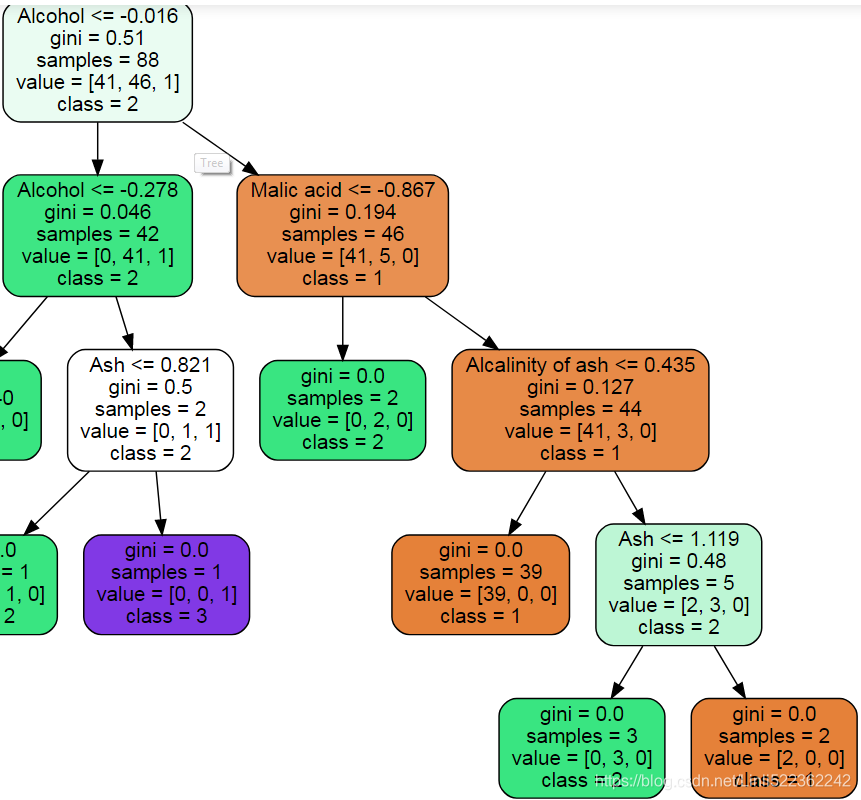
k8 = list(sbs.subsets_[8])
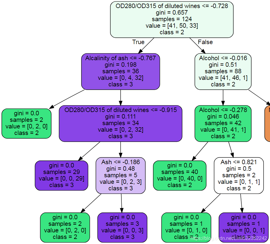
tree_clf = DecisionTreeClassifier(random_state=42)
tree_clf.fit(X_train_std[:,k8], y_train)

print('Training accuracy:', tree_clf.score(X_train_std[:,k8], y_train))
print('Test accuracy:', tree_clf.score(X_test_std[:,k8], y_test))

k8_p1 = [i+1 for i in k8]
#k8_p1 #[1, 2, 3, 4, 12]
df_wine_label=df_wine['Class label'].unique()
df_wine_label = [str(i)for i in df_wine_label]
#df_wine_label #['1', '2', '3']

# pip3 install graphviz
from graphviz import Source
from sklearn.tree import export_graphviz
import os
os.environ["PATH"] += os.pathsep + "C:/Graphviz2.38/bin" # " directory" where you intall graphviz
 
export_graphviz(
    tree_clf,
    out_file = os.path.join( "wine_tree.dot"),
    feature_names = df_wine.columns[k8_p1], ###
    class_names = df_wine_label,###
    rounded = True,
    filled = True
)
 
Source.from_file("wine_tree.dot")

all leaves' Gini impurity are 0

tree_clf.feature_importances_

k7 = list(sbs.subsets_[6])
knn.fit(X_train_std[:,k7], y_train)
print(df_wine.columns[1:][k7])
print('Training accuracy:', knn.score(X_train_std[:,k7], y_train))
print('Test accuracy:', knn.score(X_test_std[:,k7], y_test))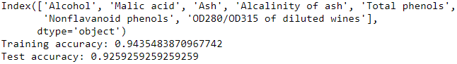

Summary: base on different classifier, the accuracy will be different. However both tree_clf and SBS can tell us that can use less features( than original dataset )

Is it possible to drop some feature columns based on the weight coefficient (if the coefficient value is 0)？
https://blog.youkuaiyun.com/Linli522362242/article/details/108230328

the answer is No:

df_wine.columns[1:][np.sum(lr.coef_, axis=0)==0.]

####################################################

Assessing feature importance with random forests

In previous sections, you learned how to use L1 regularization to zero out potentially irrelevant features via logistic regression, and use the SBS(Sequential feature selection) algorithm for feature selection and apply it to a KNN algorithm. Another useful approach to select relevant features from a dataset is to use a random forest, an ensemble technique that we introduced in Chapter 3, A Tour of Machine Learning Classifiers Using scikit-learn. Using a random forest, we can measure the feature importance as the averaged impurity decrease computed from all decision trees in the forest, without making any assumptions about whether our data is linearly separable or not. Conveniently, the random forest implementation in scikit-learn already collects the feature importance values for us so that we can access them via the feature_importances_ attribute after fitting a RandomForestClassifier. By executing the following code, we will now train a forest of 10,000 trees on the Wine dataset and rank the 13 features by their respective importance measures—remember from our discussion in Chapter 3, A Tour of Machine Learning Classifiers Using scikit-learn that we don't need to use standardized or normalized features in tree-based models:

format VS % print

from sklearn.ensemble import RandomForestClassifier
import matplotlib.pyplot as plt

feat_labels = df_wine.columns[1:]

forest = RandomForestClassifier( n_estimators=500, random_state=1 )
forest.fit(X_train, y_train)
importances = forest.feature_importances_

indices = np.argsort(importances)[::-1]

for feat in range(X_train.shape[1]):
    # % ：Placeholder(Specifier)
    # - ：Align left
    # f : float
#                         % : Delimiter    
    print("%2d) %-*s %f" % (feat+1,                      #%2d
                            30,                          #*
                            feat_labels[ indices[feat] ],#%s
                            importances[ indices[feat] ] #%f
                            )
         )
# OR
    # {} ：Placeholder( ":" : Specifier)
    # d : int
    # s : string (can be ignored)
    # < ：Align left
    # > : Align right
    # f : float
#     print("{:>2d} {:<30} {:f}".format(feat+1,                      #2d
#                             #30,                          #*
#                             feat_labels[ indices[feat] ],#%s
#                             importances[ indices[feat] ] #f
#                             )
#          )  
                
plt.title("Feature Importance")
plt.bar( range(X_train.shape[1]), importances[indices], 
         align='center')

plt.xticks(range(X_train.shape[1]), feat_labels[indices], rotation=45)
plt.xlim([-1, X_train.shape[1]])
plt.tight_layout()
plt.show()

After executing the code, we created a plot that ranks the different features in the Wine dataset, by their relative importance; note that the feature importance values are normalized so that they sum up to 1.0:

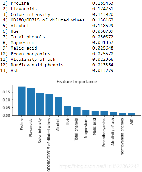
We can conclude that the proline脯氨酸 and flavonoid类黄酮 levels, the color intensity, the OD280/OD315 diffraction, and the alcohol concentration of wine are the most discriminative features in the dataset based on the average impurity decrease in the 500 decision trees. Interestingly, two of the top-ranked features in the plot are also in the three-feature subset selection from the SBS algorithm that we implemented in the previous section (alcohol concentration and OD280/OD315 of diluted wines). However, as far as interpretability is concerned, the random forest technique comes with an important gotcha that is worth mentioning. If two or more features are highly correlated, one feature may be ranked very highly while the information of the other feature(s) may not be fully captured(###Consider: decorrelation by dropping features from high correlated features###). On the other hand, we don't need to be concerned about this problem if we are merely interested in the predictive performance of a model rather than the interpretation of feature importance values.

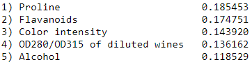
To conclude this section about feature importance values and random forests, it is worth mentioning that scikit-learn also implements a SelectFromModel object that selects features based on a user-specified threshold after model fitting, which is useful if we want to use the RandomForestClassifier as a feature selector and intermediate step in a scikit-learn Pipeline object, which allows us to connect different preprocessing steps with an estimator, as we will see in Chapter 6, Learning Best Practices for Model Evaluation and Hyperparameter Tuning. For example, we could set the threshold to 0.1 to reduce the dataset to the five most important features using the following code:

from sklearn.feature_selection import SelectFromModel
sfm = SelectFromModel( forest, threshold=0.1, prefit=True)######
X_selected = sfm.transform(X_train)
print('Number of features that meet this threshold criterion:',
      X_selected.shape[1])

# forest = RandomForestClassifier( n_estimators=500, random_state=1 )
# forest.fit(X_train, y_train)
# importances = forest.feature_importances_

for feat in range(X_selected.shape[1]):
    print("%2d) %-*s %f" % (feat+1, 
                            30, 
                            feat_labels[indices[feat]], # feat_labels = df_wine.columns[1:]
                            importances[indices[feat]]
                           )
         )

Summary

We started this chapter by looking at useful techniques to make sure that we handle missing data correctly. Before we feed data to a machine learning algorithm, we also have to make sure that we encode categorical variables correctly, and we have seen how we can map ordinal and nominal feature values to integer representations.

Moreover, we briefly discussed L1 regularization, which can help us to avoid overfitting by reducing the complexity of a model. As an alternative approach to removing irrelevant features, we used a sequential feature selection algorithm to select meaningful features from a dataset.

In the next chapter, you will learn about yet another useful approach to dimensionality reduction: feature extraction. It allows us to compress features onto a lower-dimensional subspace, rather than removing features entirely as in feature selection.