cp5_Compressing Data via Dimensionality Reduction_feature extraction_PCA_LDA_convergence_kernel PCA

     In cp4, Building Good Training Sets – Data Preprocessing, you learned about the different approaches for reducing the dimensionality of a dataset using different feature selection techniques. An alternative approach to feature selection for dimensionality reduction is feature extraction. In this chapter, you will learn about three fundamental techniques that will help us to summarize the information content of a dataset by transforming it onto a new feature subspace of lower dimensionality than the original one. Data compression is an important topic in machine learning, and it helps us to store and analyze the increasing amounts of data that are produced and collected in the modern age of technology.

In this chapter, we will cover the following topics:

• Principal Component Analysis (PCA) for unsupervised data compression
• Linear Discriminant判别式 Analysis (LDA) as a supervised dimensionality reduction technique for maximizing class separability可分离性
• Nonlinear dimensionality reduction via Kernel Principal Component Analysis (KPCA)

Unsupervised dimensionality reduction via principal component analysis

     Similar to feature selection, we can use different feature extraction techniques to reduce the number of features in a dataset. The difference between feature selection and feature extraction提取 is that while we maintain the original features when we used feature selection algorithms, such as sequential backward selection, we use feature extraction to transform or project the data onto a new feature space. In the context of dimensionality reduction, feature extraction can be understood as an approach to data compression with the goal of maintaining most of the relevant information. In practice, feature extraction is not only used to improve storage space or the computational efficiency of the learning algorithm, but can also improve the predictive performance by reducing the curse of dimensionality—especially if we are working with non-regularized models.

The main steps behind principal component analysis

     In this section, we will discuss PCA (Principal Component Analysis), an unsupervised linear transformation technique that is widely used across different fields, most prominently for feature extraction and dimensionality reduction. Other popular applications of PCA include
exploratory data analyses and de-noising去噪 of signals in stock market trading, and the analysis of genome data and gene expression levels in the field of bioinformatics生物信息学.

     PCA helps us to identify patterns in data based on the correlation between features. In a nutshell简言之, PCA aims to find the directions of maximum variance in highdimensional data and projects it onto a new subspace with equal or fewer dimensions than the original one. The orthogonal axes (principal components) of the new subspace can be interpreted as the directions of maximum variance given the constraint that the new feature axes are orthogonal to each other, as illustrated in the following figu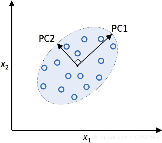re:
Here, and are the original feature axes, and PC1 and PC2 are the principal components.

######################################
   
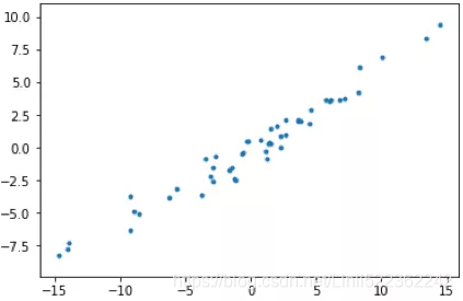
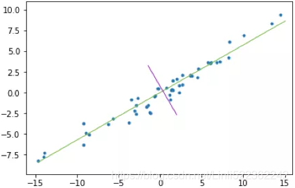
上图（左）是二维空间中经过中心化的一组数据，我们很容易看出主成分所在的轴（以下称为主轴）的大致方向，即右图中绿线所处的轴。因为在绿线所处的轴上，数据分布的更为分散，这也意味着数据在这个方向上方差更大。在信号处理领域中我们认为信号具有较大方差，噪声具有较小方差，信号与噪声之比称为信噪比，信噪比越大意味着数据的质量越好。由此我们不难引出PCA的目标，即最大化投影方差，也就是让数据在主轴上投影的方差最大。variance measures the spread of values along a feature axis. 
      It seems reasonable to select the axis that preserves the maximum amount of variance, as it will most likely lose less information than the other projections. Another way to justify this choice is that it is the axis that minimizes the mean squared distance between the original dataset and its projection onto that axis. This is the rather simple idea behind PCA.

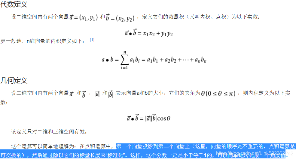
点积在数学中，又称数量积（dot product; scalar product）

a·b=（a^T）*b，这里的a^T指示矩阵a的转置。

Maximum variance formulation  08_Dimensionality Reduction_svd_Kernel_pca_make_swiss_roll_subplot2grid_IncrementalPCA_memmap_LLE_Linli522362242的专栏-优快云博客
######################################

     If we use PCA for dimensionality reduction, we construct a –dimensional transformation matrix W that allows us to map a sample vector x onto a new k–dimensional feature subspace that has fewer dimensions than the original d–dimensional feature space(k<d):

     As a result of transforming the original d-dimensional data onto this new k-dimensional subspace (typically k << d), the first principal component will have the largest possible variance, and all consequent principal components will have the largest variance given the constraint that these components are uncorrelated (orthogonal) to the other principal components—even if the input features are correlated, the resulting principal components will be mutually orthogonal (uncorrelated). Note that the PCA directions are highly sensitive to data scaling, and we need to standardize the features prior to PCA if the features were measured on different scales and we want to assign equal importance to all features.

     Before looking at the PCA algorithm for dimensionality reduction in more detail, let's summarize the approach in a few simple steps:

1. Standardize the d-dimensional dataset.
2. Construct the covariance matrix.
3. Decompose分解 the covariance matrix into its eigenvectors(principal components) and eigenvalues.
4. Sort the eigenvalues by decreasing order to rank the corresponding eigenvectors.
5. Select k eigenvectors which correspond to the k largest eigenvalues, where k is the dimensionality of the new feature subspace ( ).
6. Construct a projection matrix W from the "top" k eigenvectors.
7. Transform the d-dimensional input dataset X using the projection matrix W to obtain the new k-dimensional feature subspace.

In the following sections, we will perform a PCA step by step, using Python as a learning exercise. Then, we will see how to perform a PCA more conveniently using scikit-learn.

Total and explained variance

     In this subsection, we will tackle the first four steps of a PCA (principal component analysis):

1. standardizing the data,
2. constructing the covariance matrix,
3. obtaining the eigenvalues and eigenvectors of the covariance matrix,
4. and sorting the eigenvalues by decreasing order to rank the eigenvectors.

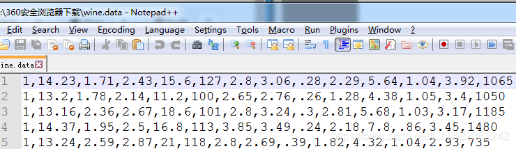
https://archive.ics.uci.edu/ml/machine-learning-databases/wine/wine.data

Data Set Information:

These data are the results of a chemical analysis of wines grown in the same region in Italy but derived from three different cultivars. The analysis determined the quantities of 13 constituents found in each of the three types of wines.

I think that the initial data set had around 30 variables, but for some reason I only have the 13 dimensional version. I had a list of what the 30 or so variables were, but a.) I lost it, and b.), I would not know which 13 variables are included in the set.

The attributes are (dontated by Riccardo Leardi, riclea '@' anchem.unige.it )
1) Alcohol
2) Malic acid
3) Ash
4) Alcalinity of ash
5) Magnesium
6) Total phenols
7) Flavanoids
8) Nonflavanoid phenols
9) Proanthocyanins
10)Color intensity
11)Hue
12)OD280/OD315 of diluted wines
13)Proline

     First, we will start by loading the Wine dataset that we have been working with in Chapter 4, Building Good Training Sets – Data Preprocessing:

import pandas as pd

df_wine = pd.read_csv('https://archive.ics.uci.edu/ml/machine-learning-databases/wine/wine.data', header=None)

df_wine.head()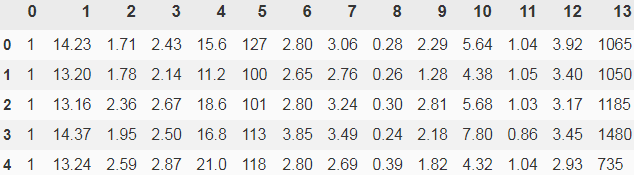

     Next, we will process the Wine data into separate training and test sets—using 70 percent and 30 percent of the data, respectively—and standardize it to unit variance:

from sklearn.model_selection import train_test_split

X,y = df_wine.iloc[:,1:].values, df_wine.iloc[:,0].values
X_train, X_test, y_train, y_test = train_test_split(X,y, test_size=0.3, stratify=y, random_state=0)

standardize the features(the PCA directions are highly sensitive to data scaling, and we need to standardize the features prior to PCA if the features were measured on different scales and we want to assign equal importance to all features.)

# standardize the features
from sklearn.preprocessing import StandardScaler

sc = StandardScaler()
X_train_std = sc.fit_transform(X_train)
X_test_std = sc.transform(X_test)

     After completing the mandatory强制的 preprocessing steps by executing the preceding code, let's advance to the second step: constructing the covariance matrix. The symmetric d × d -dimensional covariance matrix, where d is the number of dimensions in the dataset, stores the pairwise成对地 covariances between the different features. For example, the covariance between two features and on the population level can be calculated via the following equation:
    VS  sample covariances
     The reason the sample covariance matrix has N-1 in the denominator rather than N is essentially that the population mean(OR u) is not known and is replaced by the sample mean . 
     Here, and are the sample means of feature j and k , respectively. Note that the sample means are zero if we standardize the dataset. A positive covariance between two features indicates that the features increase or decrease together, whereas a negative covariance indicates that the features vary in opposite directions. For example, a covariance matrix of three features can then be written as (note that  stands for the Greek uppercase letter sigma, which is not to be confused with the sum symbol):

08_09_Dimension Reduction_Gaussian mixture_kmeans++_extent_tick_params_silhouette_image segment_tSNE_Linli522362242的专栏-优快云博客
     The eigenvectors of the covariance matrix represent the principal components (the directions of maximum variance ), whereas the corresponding eigenvalues will define their magnitude.  In the case of the Wine dataset, we would obtain 13 eigenvectors and eigenvalues from the 13×13 -dimensional covariance matrix. 

     Now, let's obtain the eigenpairs of the covariance matrix. As we surely remember from our introductory linear algebra or calculus classes, an eigen vector satisfies the following condition:

     Here, is a scalar: the eigenvalue(Lagrange multiplier). Since the manual computation of eigenvectors and eigenvalues is a somewhat tedious and elaborate复杂 task, we will use the linalg.eig function from NumPy to obtain the eigenpairs of the Wine covariance matrix:
########################################
08_Dimensionality Reduction_svd_Kernel_pca_make_swiss_roll_subplot2grid_IncrementalPCA_memmap_LLE_Linli522362242的专栏-优快云博客

12.1.1 Maximum variance formulation

     Consider a data set of observations  where n = 1, . . . , N, and  is a Euclidean variable with dimensionality D. Our goal is to project the data onto a space having dimensionality M <D while maximizing the variance of the projected data. For the moment, we shall assume that the value of M is given. Later in this chapter, we shall consider techniques to determine an appropriate value of M from the data.

     To begin with, consider the projection onto a one-dimensional space (M = 1). We can define the direction of this space using a D-dimensional vector , which for convenience (and without loss of generality) we shall choose to be a unit vector so that  = 1 (note that we are only interested in the direction defined by , not in the magnitude of  itself). Each data point  is then projected onto a scalar value . The mean of the projected data is  where  is the sample set mean given by (12.1)

and the variance of the projected data is given by  (12.2)
where S is the data covariance 协方差 matrix defined by (12.3)

     We now maximize the projected variance  with respect to . Clearly, this has to be a constrained maximization to prevent . The appropriate constraint comes from the normalization condition归一化条件  = 1. To enforce this constraint, we introduce a Lagrange multiplier that we shall denote by , and then make an unconstrained maximization of  (12.4)

     By setting the derivative with respect to  equal to zero, we see that this quantity will have a stationary point驻点 when  (12.5)            which says that must be an eigenvector 特征向量 of S. If we left-multiply by  and make use of  = 1, we see that the variance is given by  (12.6)

and so the variance will be a maximum when we set  equal to the eigenvector having the largest eigenvalue . This eigenvector is known as the first principal component.

     We can define additional principal components in an incremental fashion方式 by choosing each new direction to be that which maximizes the projected variance amongst all possible directions orthogonal to those already considered. If we consider the general case of an M-dimensional projection space, the optimal linear projection for which the variance of the projected data is maximized is now defined by the M eigenvectors  of the data covariance matrix S corresponding to the M largest eigenvalues . This is easily shown using proof by induction.
########################################

     Here, is a scalar: the eigenvalue(Lagrange multiplier). Since the manual computation of eigenvectors and eigenvalues is a somewhat tedious and elaborate复杂 task, we will use the linalg.eig function from NumPy to obtain the eigenpairs of the Wine covariance matrix:

import numpy as np

cov_mat = np.cov(X_train_std.T) #the covariance matrix
eigen_vals, eigen_vecs = np.linalg.eig( cov_mat )
print('\nEigenValues \n%s' % eigen_vals)

 
     Using the numpy.cov function, we computed the covariance matrix of the standardized training dataset. Using the linalg.eig function, we performed the eigen decomposition, which yielded a vector (eigen_vals) consisting of 13 eigenvalues and the corresponding eigenvectors stored as columns in a 13 x 13-dimensional matrix (eigen_vecs).
####################################################

Note

     The numpy.linalg.eig function was designed to operate on both symmetric and non-symmetric square matrices. However, you may find that it returns complex（复合） eigenvalues in certain cases.

     A related function, numpy.linalg.eigh, has been implemented to decompose Hermetian matrices, which is a numerically more stable approach to work with symmetric matrices such as the covariance matrix; numpy.linalg.eigh always returns real eigenvalues.
####################################################

Total and explained variance

     Since we want to reduce the dimensionality of our dataset by compressing it onto a new feature subspace, we only select the subset of the eigenvectors (principal components) that contains most of the information (variance方差最大). The eigenvalues define the magnitude of the eigenvectors（特征值的大小决定了特征向量的重要性）, so we have to sort the eigenvalues by decreasing magnitude; we are interested in the top k eigenvectors based on the values of their corresponding eigenvalues. But before we collect those k most informative eigenvectors, let us plot the variance explained ratios of the eigenvalues. The variance explained ratio(方差解释比率或者方差贡献率) of an eigenvalue is simply the fraction of an eigenvalue and the total sum of the eigenvalues:

     Using the NumPy cumsum function, we can then calculate the cumulative sum of explained variances, which we will then plot via Matplotlib's step function:

tot = sum(eigen_vals) #the total sum of the eigenvalues
var_exp = [ (i/tot) for i in sorted(eigen_vals, reverse=True) ] #The variance explained ratio of an eigenvalue
cum_var_exp = np.cumsum( var_exp ) #the cumulative sum of explained variances

import matplotlib.pyplot as plt

         #13 eigenvalues
plt.bar( range(1,14), var_exp, alpha=0.5, align="center", label="individual explained variance")
#where="mid": Steps occur half-way between the *x* positions.
plt.step( range(1,14), cum_var_exp, where="mid", label="cumulative explained variance")
plt.ylabel("Explained variance ratio")
plt.xlabel("Principal component index")
plt.legend(loc="best")
plt.show()

     The resulting plot indicates that the first principal component alone accounts for approximately 40 percent of the variance. Also, we can see that the first two principal components combined explain almost 60 percent of the variance in the dataset:

    Although the explained variance plot reminds us of the feature importance values that we computed in Chapter 4, Building Good Training Sets – Data Preprocessing, via random forests, we should remind ourselves that PCA is an unsupervised method, which means that information about the class labels is ignored. Whereas a random forest uses the class membership information to compute the node impurities, variance measures the spread of values along a feature axis.

Feature transformation

     After we have successfully decomposed the covariance matrix into eigenpairs(eigenvector and eigenvalue), let's now proceed with the last three steps to transform the Wine dataset onto the new principal component axes. The remaining steps we are going to tackle in this section are the following ones:

• Select k eigenvectors, which correspond to the k largest eigenvalues, where k is the dimensionality of the new feature subspace ( ).
• Construct a projection matrix W from the "top" k eigenvectors.
• Transform the d-dimensional input dataset X using the projection matrix W to obtain the new k-dimensional feature subspace.

     Or, in less technical terms, we will sort the eigenpairs by descending order of the eigenvalues, construct a projection matrix from the selected eigenvectors, and use the projection matrix to transform the data onto the lower-dimensional subspace.

We start by sorting the eigenpairs by decreasing order of the eigenvalues:

# Make a list of (eigenvalue, eigenvector) tuples
eigen_pairs = [ (np.abs(eigen_vals[i]), eigen_vecs[:,i]) for i in range(len(eigen_vals)) ]
eigen_pairs.sort(reverse=True)

     Next, we collect the two eigenvectors that correspond to the two largest eigenvalues, to capture about 60 percent of the variance in this dataset. Note that we only chose two eigenvectors for the purpose of illustration, since we are going to plot the data via a two-dimensional scatter plot later in this subsection. In practice, the number of principal components has to be determined by a trade-off between computational efficiency and the performance of the classifier:

eigen_pairs[:2]

#eigen_pairs:[(eigen_value, eigen_vector(array type)),
#             (eigen_value, eigen_vector),...]             
              #eigen_pairs[0][1]: get first eigenvector or first principal component
w = np.hstack((eigen_pairs[0][1][:, np.newaxis],#[:, np.newaxis]:the principal component as 1st column
               eigen_pairs[1][1][:, np.newaxis] #[:, np.newaxis]:the principal component as 2nd column
              )
             )#( ([1st column], [second column]) )
print('Matrix W:\n', w)

By executing the preceding code, we have created a 13 x 2-dimensional projection matrix W from the top two eigenvectors.
#########################################
Note

     Depending on which version of NumPy and LAPACK(Linear Algebra PACKage) you are using, you may obtain the matrix W with its signs flipped. Please note that this is not an issue; if v is an eigenvector of a (covariance) matrix , we have:

Here is our eigenvalue, and - is also an eigenvector( and v is a unit vector, note that we are only interested in the direction defined by v) that has the same eigenvalue, since:

#########################################
     Using the projection matrix, we can now transform a sample x (represented as a 1 x 13-dimensional row) onto the PCA subspace (the principal components one and two) obtaining , now a two-dimensional sample vector consisting of two new features:

X_train_std[0].dot(w)

     Similarly, we can transform the entire 124 x 13-dimensional training dataset onto the two principal comp