


该文主要内容为一个完整神经网络的代码实现
1 神经网络的主要过程有:
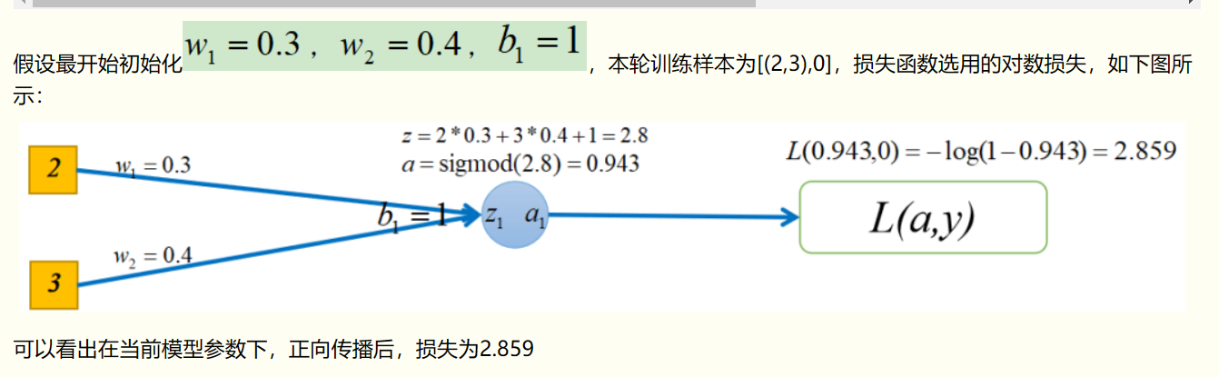
1.1 前馈过程或者叫正向传播
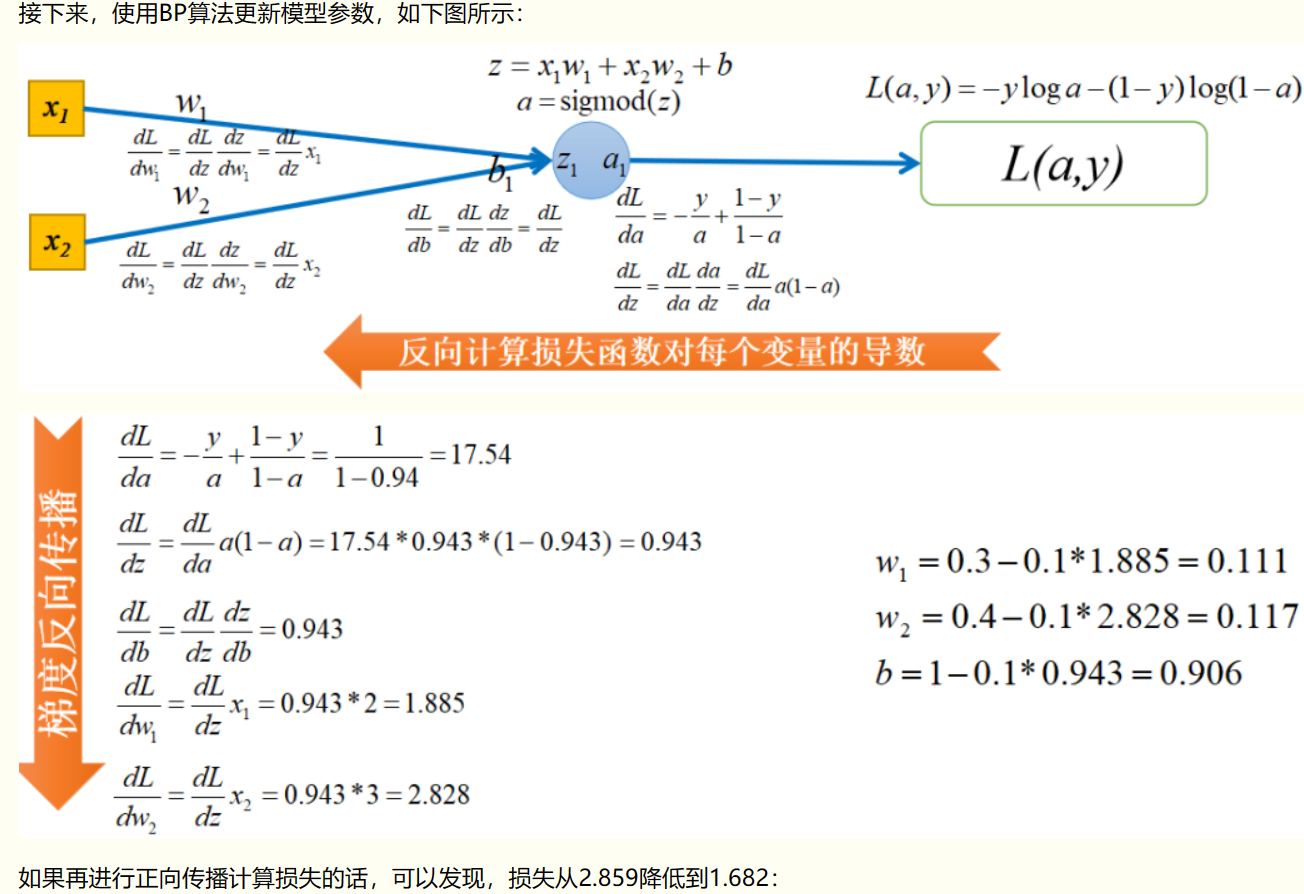
1.2 误差反传或者叫反向传播
1.3 设置迭代次数训练模型
1.4 设置评价指标,生成评价指标
2 正向传播图示(仅供参考)与代码:
注:正向传播较容易理解,无非是每层都进行:权重*输入+偏移项,再使用激活函数计算后作为下一层的输入
def __init__(self, layer_list=[], lr=0.1, epochs=100):
    self.lr = lr                    #学习率
    self.layer_list = layer_list    # 每层神经元(节点)个数
    self.epochs = epochs            #迭代次数

# 超参初始化
def weight_bias_init(self):
    self.W = {}     #权重字典,key是层号,value是对应权重矩阵
    self.b = {}     #偏置字典,key是层号,value是对应偏置矩阵

    self.layer_num = len(self.layer_list)-1 #网络层数(权重矩阵的个数,输入层无权重)
    for idx in range(self.layer_num):       #为每层layer初始化W与b矩阵,每层 W 的shape为(前一层神经元个数,后一层神经元个数)
        self.W[idx] = np.random.randn(self.layer_list[idx], \
                          self.layer_list[idx+1]) * 0.01 #正态分布
        self.b[idx] = np.random.randn(self.layer_list[idx+1])
def forward(self, X, y):
        self.X = X  #将输入X保存为类的属性,可供其他函数使用
        self.y = np.array(y).reshape(-1, 1) #更改y的shape,防止运算出错

        #记录各层的z与a,反向传播时会用到
        self.z = {}  #字典,记录每层激活前的输出(z = W*X + b)
        self.a = {}  #字典,记录每层激活后的输出(a = sigmoid(z))

        input = self.X
        for idx in range(self.layer_num):  #循环向前累乘
            self.z[idx] = np.dot(input, self.W[idx]) + self.b[idx]  #z = W*X + b
            self.a[idx] = self.sigmoid(self.z[idx])                 #a = sigmoid(z)
            input = self.a[idx]            #更新输入

        self.output = self.a[self.layer_num-1]    #记录最后一层输出
        self.loss = -np.mean(self.y * np.log(self.output) + \
                        (1-self.y) * np.log(1-self.output))  #对数损失
3 反向传播图示以及代码
关于反向传播该图仅作为参考之一,如果有困惑可以详细看参考资料,反向传播为该内容的核心和难点。
# sigmoid的一阶导数
def Dsigmoid(self, x):
    return self.sigmoid(x) * (1 - self.sigmoid(x))
# 反向传播
def backward(self):
    #跟权重保存方式一样,使用字典存储,key为对应的层号
    self.dz = {}    #对每层z的求导
    self.dW = {}    #对每层W的求导
    self.db = {}    #对每层b的求导

    idx = self.layer_num - 1    #从后往前求导
    while(idx>=0):
        #********** 求dz *********#
        if(idx==self.layer_num-1): #最后一层的求导比较特殊,套最后一层求导的公式dz3
            self.dz[idx] = (self.output-self.y) * self.Dsigmoid(self.z[idx])  #元素乘
        else:                      #前层都可根据最后一层的dz迭代得到,套迭代公式dzi
            self.dz[idx] = np.dot(self.dz[idx+1], self.W[idx+1].T) \
                * self.Dsigmoid(self.z[idx])

        #********** 求dW *********#
        if(idx == 0):  #idx为0时,即到达第一层时,前层输入a[idx-1]是X
            self.dW[idx] = np.dot(self.X.T, self.dz[idx]) / len(self.X) #梯度需除上总样本数
        else:          #idx不为0时迭代计算即可
            self.dW[idx] = np.dot(self.a[idx-1].T, self.dz[idx]) / len(self.X)

        #********** 求db *********#
        self.db[idx] = np.sum(self.dz[idx], axis=0) / len(self.X) #db=dz, 但是需要所有维度取平均
        idx -= 1    #跳前一层

    # 求完所有层的梯度后,更新即可
    for idx in range(self.layer_num):
        self.W[idx] -= self.lr * self.dW[idx]
        self.b[idx] -= self.lr * self.db[idx]
4 完整代码1展示:
上述代码以及接下来的完整代码1可以参考此处:
import numpy as np
class NN(object):
def __init__(self, layer_list=[], lr=0.1, epochs=100):
self.lr = lr #学习率
self.layer_list = layer_list #每层神经元个数
self.epochs = epochs #迭代次数
#权重与偏执初始化
def weight_bias_init(self):
self.W = {} #权重字典,key是层号,value是权重矩阵
self.b = {} #偏置字典,key是层号,value是怕偏置矩阵
self.layer_num = len(self.layer_list)-1 #网络层数
#为每层layer初始化W与b矩阵
for idx in range(self.layer_num):
self.W[idx] = np.random.randn(self.layer_list[idx], \
self.layer_list[idx+1]) * 0.01 #正态分布
self.b[idx] = np.random.randn(self.layer_list[idx+1])
# sigmoid函数
def sigmoid(self, x):
return 1.0 / (1 + np.exp(-x))
# sigmoid的一阶导数
def Dsigmoid(self, x):
return self.sigmoid(x) * (1 - self.sigmoid(x))
# 前向传播
def forward(self, X, y):
self.X, self.y = X, np.array(y).reshape(-1, 1)
self.z = {} #记录每层激活前的输出(z = W*X + b)
self.a = {} #记录每层激活后的输出(a = sigmoid(z))
#循环向前累乘
input = self.X
for idx in range(self.layer_num):
self.z[idx] = np.dot(input, self.W[idx]) + self.b[idx]
self.a[idx] = self.sigmoid(self.z[idx])
input = self.a[idx] #更新输入
self.output = self.a[self.layer_num-1] #最后一层输出
self.loss = -np.mean(self.y * np.log(self.output) + \
(1-self.y) * np.log(1-self.output)) #对数损失
#误差反向传播
def backward(self):
#跟权重保存方式一样,使用字典存储,key为对应的层号
self.dz = {} #对每层z的求导
self.dW = {} #对每层W的求导
self.db = {} #对每层b的求导
idx = self.layer_num - 1 #从后往前求导
while(idx>=0):
#********** 求dz *********#
if(idx==self.layer_num-1): #最后一层的求导比较特殊,套最后一层求导的公式dz3
self.dz[idx] = (self.output-self.y) * self.Dsigmoid(self.z[idx]) #元素乘
else: #前层都可根据最后一层的dz迭代得到,套迭代公式dzi
self.dz[idx] = np.dot(self.dz[idx+1], self.W[idx+1].T) \
* self.Dsigmoid(self.z[idx])
#********** 求dW *********#
if(idx == 0): #idx为0时,即到达第一层时,前层输入a[idx-1]是X
self.dW[idx] = np.dot(self.X.T, self.dz[idx]) / len(self.X) #梯度需除上总样本数
else: #idx不为0时迭代计算即可
self.dW[idx] = np.dot(self.a[idx-1].T, self.dz[idx]) / len(self.X)
#********** 求db *********#
self.db[idx] = np.sum(self.dz[idx], axis=0) / len(self.X) #db=dz, 但是需要所有维度取平均
idx -= 1 #跳前一层
# 求完所有层的梯度后,更新即可
for idx in range(self.layer_num):
self.W[idx] -= self.lr * self.dW[idx]
self.b[idx] -= self.lr * self.db[idx]
#迭代训练
def train(self, X, y):
self.weight_bias_init()
for i in range(self.epochs):
self.forward(X, y)
self.backward()
#每10轮打印一次loss
if(i%10==0): print("Epoch {}: loss={}".format(i//10+1, self.loss))
#预测概率输出
def predict(self, X_test):
input = X_test
for idx in range(self.layer_num):
z = np.dot(input, self.W[idx]) + self.b[idx]
a = self.sigmoid(z)
input = a
return a
from sklearn.datasets import load_iris
from sklearn.model_selection import train_test_split
from sklearn.metrics import accuracy_score
X, y = load_iris(return_X_y=True)
X, y = X[:100], y[:100]
X_train, X_test, y_train, y_test = train_test_split(X, y, test_size=0.4)
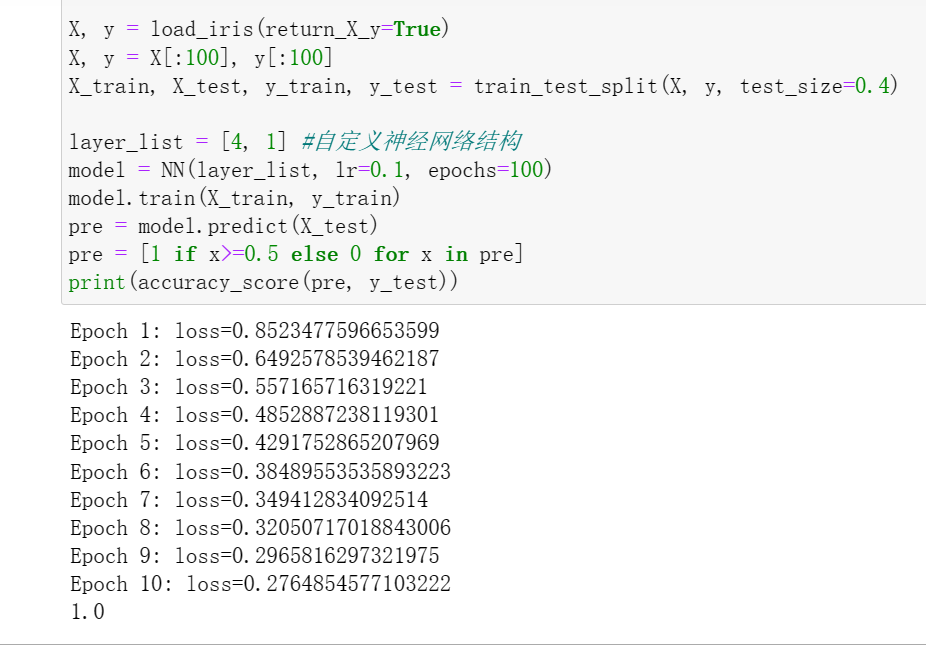
layer_list = [4, 1] #自定义神经网络结构
model = NN(layer_list, lr=0.1, epochs=100)
model.train(X_train, y_train)
pre = model.predict(X_test)
pre = [1 if x>=0.5 else 0 for x in pre]
print(accuracy_score(pre, y_test))
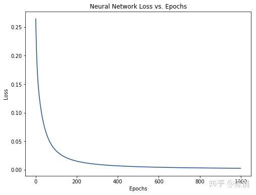
运行结果展示:
5 完整代码2展示:
import numpy as np

def sigmoid(x):
  # Sigmoid activation function: f(x) = 1 / (1 + e^(-x))
  return 1 / (1 + np.exp(-x))

def deriv_sigmoid(x):
  # Derivative of sigmoid: f'(x) = f(x) * (1 - f(x))
  fx = sigmoid(x)
  return fx * (1 - fx)

def mse_loss(y_true, y_pred):
  # y_true and y_pred are numpy arrays of the same length.
  return ((y_true - y_pred) ** 2).mean()

class OurNeuralNetwork:
  '''
  A neural network with:
    - 2 inputs
    - a hidden layer with 2 neurons (h1, h2)
    - an output layer with 1 neuron (o1)

  *** DISCLAIMER ***:
  The code below is intended to be simple and educational, NOT optimal.
  Real neural net code looks nothing like this. DO NOT use this code.
  Instead, read/run it to understand how this specific network works.
  '''
  def __init__(self):
    # 权重,Weights
    self.w1 = np.random.normal()
    self.w2 = np.random.normal()
    self.w3 = np.random.normal()
    self.w4 = np.random.normal()
    self.w5 = np.random.normal()
    self.w6 = np.random.normal()

    # 截距项,Biases
    self.b1 = np.random.normal()
    self.b2 = np.random.normal()
    self.b3 = np.random.normal()

  def feedforward(self, x):
    # x is a numpy array with 2 elements.
    h1 = sigmoid(self.w1 * x[0] + self.w2 * x[1] + self.b1)
    h2 = sigmoid(self.w3 * x[0] + self.w4 * x[1] + self.b2)
    o1 = sigmoid(self.w5 * h1 + self.w6 * h2 + self.b3)
    return o1

  def train(self, data, all_y_trues):
    '''
    - data is a (n x 2) numpy array, n = # of samples in the dataset.
    - all_y_trues is a numpy array with n elements.
      Elements in all_y_trues correspond to those in data.
    '''
    learn_rate = 0.1
    epochs = 1000 # number of times to loop through the entire dataset

    for epoch in range(epochs):
      for x, y_true in zip(data, all_y_trues):
        # --- Do a feedforward (we'll need these values later)
        sum_h1 = self.w1 * x[0] + self.w2 * x[1] + self.b1
        h1 = sigmoid(sum_h1)

        sum_h2 = self.w3 * x[0] + self.w4 * x[1] + self.b2
        h2 = sigmoid(sum_h2)

        sum_o1 = self.w5 * h1 + self.w6 * h2 + self.b3
        o1 = sigmoid(sum_o1)
        y_pred = o1

        # --- Calculate partial derivatives.
        # --- Naming: d_L_d_w1 represents "partial L / partial w1"
        d_L_d_ypred = -2 * (y_true - y_pred)

        # Neuron o1
        d_ypred_d_w5 = h1 * deriv_sigmoid(sum_o1)
        d_ypred_d_w6 = h2 * deriv_sigmoid(sum_o1)
        d_ypred_d_b3 = deriv_sigmoid(sum_o1)

        d_ypred_d_h1 = self.w5 * deriv_sigmoid(sum_o1)
        d_ypred_d_h2 = self.w6 * deriv_sigmoid(sum_o1)

        # Neuron h1
        d_h1_d_w1 = x[0] * deriv_sigmoid(sum_h1)
        d_h1_d_w2 = x[1] * deriv_sigmoid(sum_h1)
        d_h1_d_b1 = deriv_sigmoid(sum_h1)

        # Neuron h2
        d_h2_d_w3 = x[0] * deriv_sigmoid(sum_h2)
        d_h2_d_w4 = x[1] * deriv_sigmoid(sum_h2)
        d_h2_d_b2 = deriv_sigmoid(sum_h2)

        # --- Update weights and biases
        # Neuron h1
        self.w1 -= learn_rate * d_L_d_ypred * d_ypred_d_h1 * d_h1_d_w1
        self.w2 -= learn_rate * d_L_d_ypred * d_ypred_d_h1 * d_h1_d_w2
        self.b1 -= learn_rate * d_L_d_ypred * d_ypred_d_h1 * d_h1_d_b1

        # Neuron h2
        self.w3 -= learn_rate * d_L_d_ypred * d_ypred_d_h2 * d_h2_d_w3
        self.w4 -= learn_rate * d_L_d_ypred * d_ypred_d_h2 * d_h2_d_w4
        self.b2 -= learn_rate * d_L_d_ypred * d_ypred_d_h2 * d_h2_d_b2

        # Neuron o1
        self.w5 -= learn_rate * d_L_d_ypred * d_ypred_d_w5
        self.w6 -= learn_rate * d_L_d_ypred * d_ypred_d_w6
        self.b3 -= learn_rate * d_L_d_ypred * d_ypred_d_b3

      # --- Calculate total loss at the end of each epoch
      if epoch % 10 == 0:
        y_preds = np.apply_along_axis(self.feedforward, 1, data)
        loss = mse_loss(all_y_trues, y_preds)
        print("Epoch %d loss: %.3f" % (epoch, loss))

# Define dataset
data = np.array([
  [-2, -1],  # Alice
  [25, 6],   # Bob
  [17, 4],   # Charlie
  [-15, -6], # Diana
])
all_y_trues = np.array([
  1, # Alice
  0, # Bob
  0, # Charlie
  1, # Diana
])

# Train our neural network!
network = OurNeuralNetwork()
network.train(data, all_y_trues)
# Make some predictions
emily = np.array([-7, -3]) # 128 pounds, 63 inches
frank = np.array([20, 2])  # 155 pounds, 68 inches
print("Emily: %.3f" % network.feedforward(emily)) # 0.951 - F
print("Frank: %.3f" % network.feedforward(frank)) # 0.039 - M
注:代码1主要是用矩阵的方式实现,虽然易于理解但是从公式到代码实现,代码2更丝滑一些,代码2理解后再去理解代码1,后续大多深度学习场景都会是矩阵形式。
6 参考资料:
1 该文承接前两篇文章,都为对下面文章的总结,但是该文章代码部分第一为python2实现,第二 个人无法理解参透,所以该文代码部分为另外文章所给:
参考文章1
2 关于代码1和2可以分别参考一下两篇文章,带入原作者思路,不理解的地方继续看参考资料
代码1
代码2
3 关于反向传播的理解,在两个代码文章中都有些抽象,可以配合一下文章理解
公式详解


 8605
8605

 被折叠的 条评论
为什么被折叠?
被折叠的 条评论
为什么被折叠?
 到【灌水乐园】发言


