【WY】数据处理 — Python 阶段一：基础语法八 —— 分类分析：KNN最邻近分类

本文链接：https://blog.youkuaiyun.com/InitialHeart2021/article/details/122187320

文章目录

一、基础理论
二、代码实现

一、基础理论

1.1 分类分析

在这里插入图片描述

1.2 KNN最邻近分类算法

在这里插入图片描述

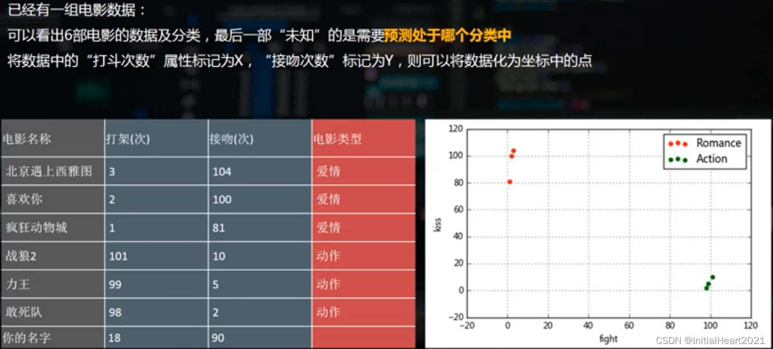
1.2.1 案例分析

在这里插入图片描述

二、代码实现

最邻近分类算法，故名思意就是在距离空间里，如果一个样本的最接近的k个邻居里绝大多数属于某个类别，则该样本也属于这个类别。

import numpy as np
import pandas as pd
import matplotlib.pyplot as plt
%matplotlib inline

# 步骤一（替换sans-serif字体）
plt.rcParams['font.sans-serif'] = ['SimHei']

# 步骤二（解决坐标轴负数的负号显示问题
plt.rcParams['axes.unicode_minus'] = False

2.1 电影分类

# 导入 KNN 分类模块
from sklearn import neighbors

# 不发出警告
import warnings
warnings.filterwarnings('ignore')

data = {
    'name':['北京遇上西雅图','喜欢你','疯狂动物城','战狼','力王','敢死队'],
    'fight':[3,2,1,101,99,98],
    'kiss':[104,100,81,10,5,2],
    'type':['Romance','Romance','Romance','Action','Action','Action']
}
data = pd.DataFrame(data)


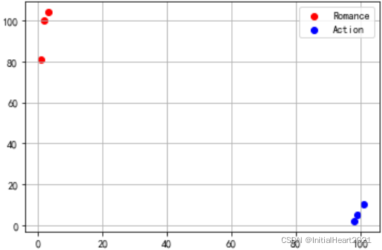
# 散点图
plt.scatter(data[data['type'] == 'Romance']['fight'], data[data['type'] == 'Romance']['kiss'], color = 'r', label = 'Romance')
plt.scatter(data[data['type'] == 'Action']['fight'], data[data['type'] == 'Action']['kiss'], color = 'b', label = 'Action')
plt.legend()
plt.grid()

2.1.1 预测1：（18, 90）属于哪一类

# 通过原始时间我们可以清楚的看出他们的特征

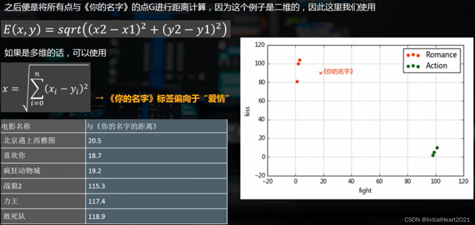
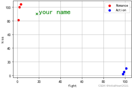
# 这时我们对[18,90]打架次数为 18，接吻次数为 90的《你的名字》用 KNN 算法进行预测

# 建立 KNN 模型

knn = neighbors.KNeighborsClassifier()

knn.fit(data[['fight', 'kiss']], data['type'])

# 预测
knn.predict([[18, 90]])   # array(['Romance'], dtype=object)：预测结果为爱情片

array(['Romance'], dtype=object)

# 散点图
plt.scatter(data[data['type'] == 'Romance']['fight'], data[data['type'] == 'Romance']['kiss'], color = 'r', label = 'Romance')
plt.scatter(data[data['type'] == 'Action']['fight'], data[data['type'] == 'Action']['kiss'], color = 'b', label = 'Action')
plt.legend()
plt.grid()

plt.scatter(18, 90, marker = 'x', color = 'g', label = 'Romance')
plt.xlabel('fight')
plt.ylabel('kiss')
plt.text(20, 90, 'your name', color = 'g', fontsize = 20)

2.1.1 预测2：创建更多的实例数据进行预测

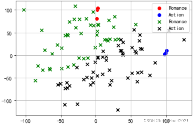
# 我们通过散点图也可以清楚的看到预测的结果

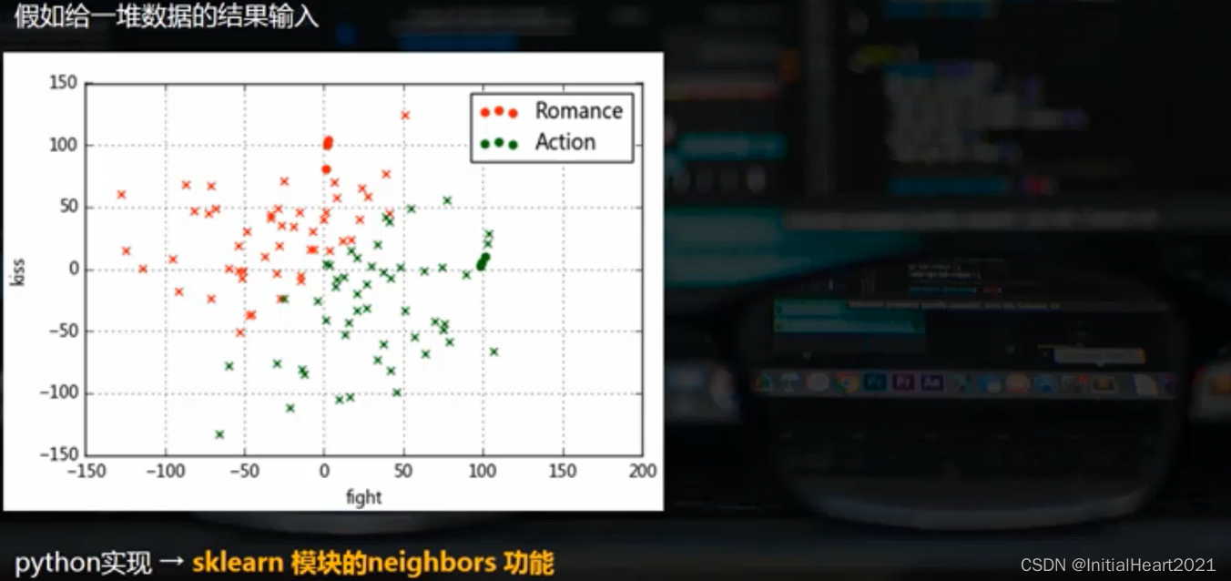
# 我们建立更多数据通过训练 KNN 模型对其预测，并通过散点图直观看他的结果

data_2 = np.random.randn(100, 2) * 50

data_2 = pd.DataFrame(data_2, columns = ['fight', 'kiss'])


# 预测
data_2['predict'] = knn.predict(data_2[['fight', 'kiss']])

# 散点图
plt.scatter(data[data['type'] == 'Romance']['fight'], data[data['type'] == 'Romance']['kiss'], color = 'r', label = 'Romance')
plt.scatter(data[data['type'] == 'Action']['fight'], data[data['type'] == 'Action']['kiss'], color = 'b', label = 'Action')
plt.legend()
plt.grid()



plt.scatter(data_2[data_2['predict'] == 'Romance']['fight'], data_2[data_2['predict'] == 'Romance']['kiss'], color = 'g', marker = 'x', label = 'Romance')
plt.scatter(data_2[data_2['predict'] == 'Action']['fight'], data_2[data_2['predict'] == 'Action']['kiss'], color = 'k', marker = 'x', label = 'Action')
plt.legend(loc = 'upper right')

# 圆点为用于训练模型的6个数据，x点为新建数据

2.2 植物分类

# 这里调用sklearn中的datasets官方数据，并把它转成pandas的Dataframe

from sklearn import datasets

# 导入官方数据
iris = datasets.load_iris()

print(iris.keys())

# 查看数据长度
print('数据长度：%i' % (len(iris['data'])))

print(iris.feature_names)
print(iris.target_names)

print(iris.data[:5])

运行结果

dict_keys(['data', 'target', 'target_names', 'DESCR', 'feature_names'])

数据长度：150

['sepal length (cm)', 'sepal width (cm)', 'petal length (cm)', 'petal width (cm)']

['setosa' 'versicolor' 'virginica']

[[5.1 3.5 1.4 0.2]
 [4.9 3.  1.4 0.2]
 [4.7 3.2 1.3 0.2]
 [4.6 3.1 1.5 0.2]
 [5.  3.6 1.4 0.2]]

# 150个实例数据
# feature_names 特征分类：萼片长度 萼片宽度 花瓣长度 花瓣宽度
# 目标类别 ['setosa' 'versicolor' 'virginica']

data = pd.DataFrame(iris.data, columns = iris.feature_names)
data['target'] = iris.target

# 通过 merge 添加类别名称

ty = {
    'target': [0, 1, 2],
    'target_names': ['setosa','versicolor','virginica']
}

ty = pd.DataFrame(ty)

data = pd.merge(data, ty, on = 'target')

# 影响类别的四个特征[‘sepal length (cm)’, ‘sepal width (cm)’, ‘petal length (cm)’, ‘petal width (cm)’]

# 我们对原数据训练，并预测四个特征依此为[0.2,0.1,0.3,0.4]的植物类别

# 建立 KNN 分类模型
knn = neighbors.KNeighborsClassifier()

# 参数(特征，类别)
knn.fit(iris.data, data['target_names'])

# 预测
pre_data = knn.predict([[0.2,0.1,0.3,0.4]])

print(pre_data)   # ['setosa']：预测结果为setosa(刺芒野古草)

['setosa']

data

运行结果

   sepal length (cm)  sepal width (cm)   petal length (cm)    petal width (cm)	target	  target_names
0	            5.1	               3.5	              1.4	              0.2	     0	        setosa
1	            4.9	               3.0	              1.4	              0.2	     0	        setosa
2	            4.7	               3.2	              1.3	              0.2	     0	        setosa
3	            4.6	               3.1	              1.5	              0.2	     0	        setosa
4	            5.0	               3.6	              1.4	              0.2	     0	        setosa
...	...	...	...	...	...	...
145	            6.7	               3.0                5.2	              2.3	     2	     virginica
146	            6.3	               2.5	              5.0	              1.9	     2	     virginica
147	            6.5	               3.0	              5.2	              2.0	     2	     virginica
148	            6.2	               3.4	              5.4	              2.3	     2	     virginica
149	            5.9	               3.0	              5.1           	  1.8	     2	     virginica

150 rows × 6 columns