


 本文介绍了Python中的PCA主成分分析和K-means聚类算法。PCA作为数据降维的方法,通过线性变换降低高维数据到低维空间,而K-means是一种基于距离的聚类算法,用于将数据点分成多个簇。文章涵盖了PCA的基本理论、降维应用以及K-means的实现逻辑和注意事项。
版权声明:本文为博主原创文章,未经博主允许不得转载。
文章目录
一、基础理论
1.1 聚类分析
1.1.1 介绍

1.1.2 分类
1.2 矩阵分解
1.2.1 分类
1.2.1.1 PCA主成分分析
1.2.1.1.1 介绍

1.2.1.1.2 目的
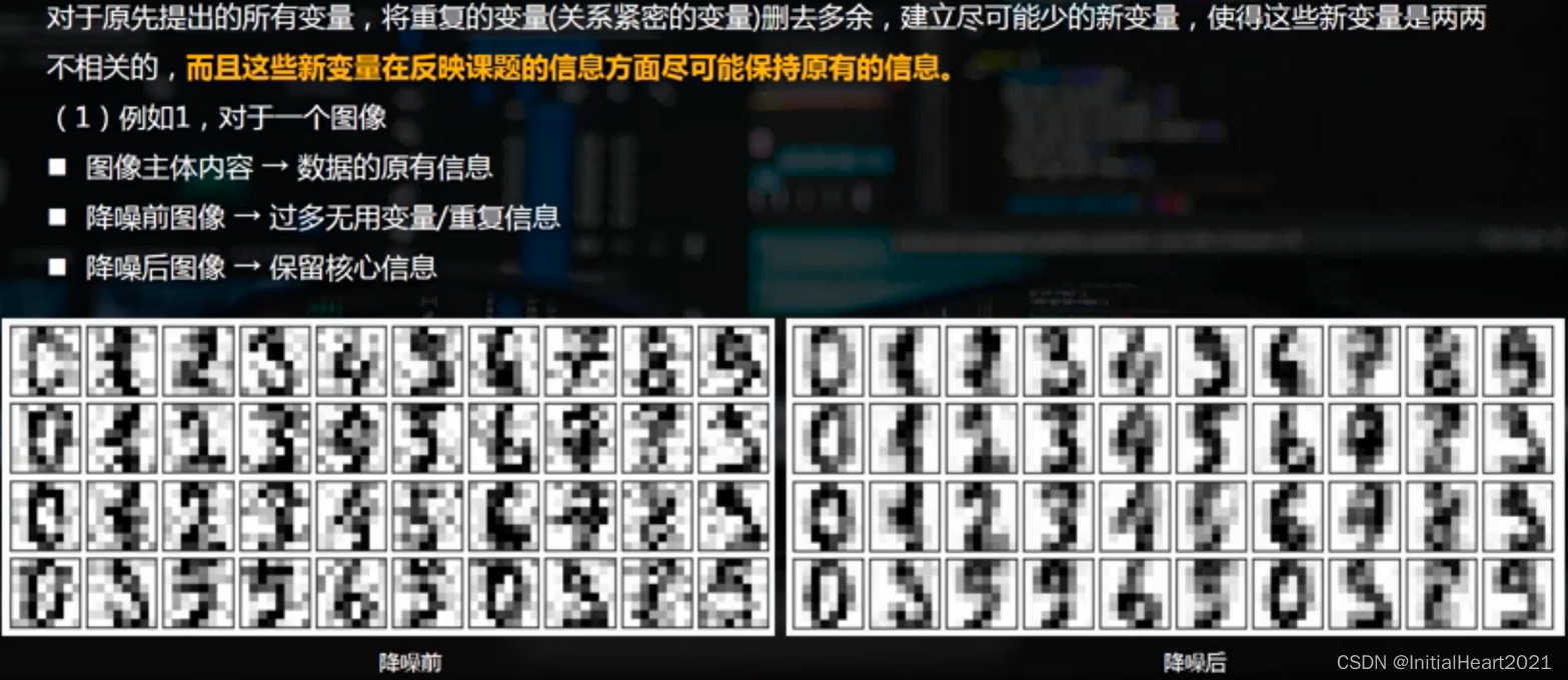
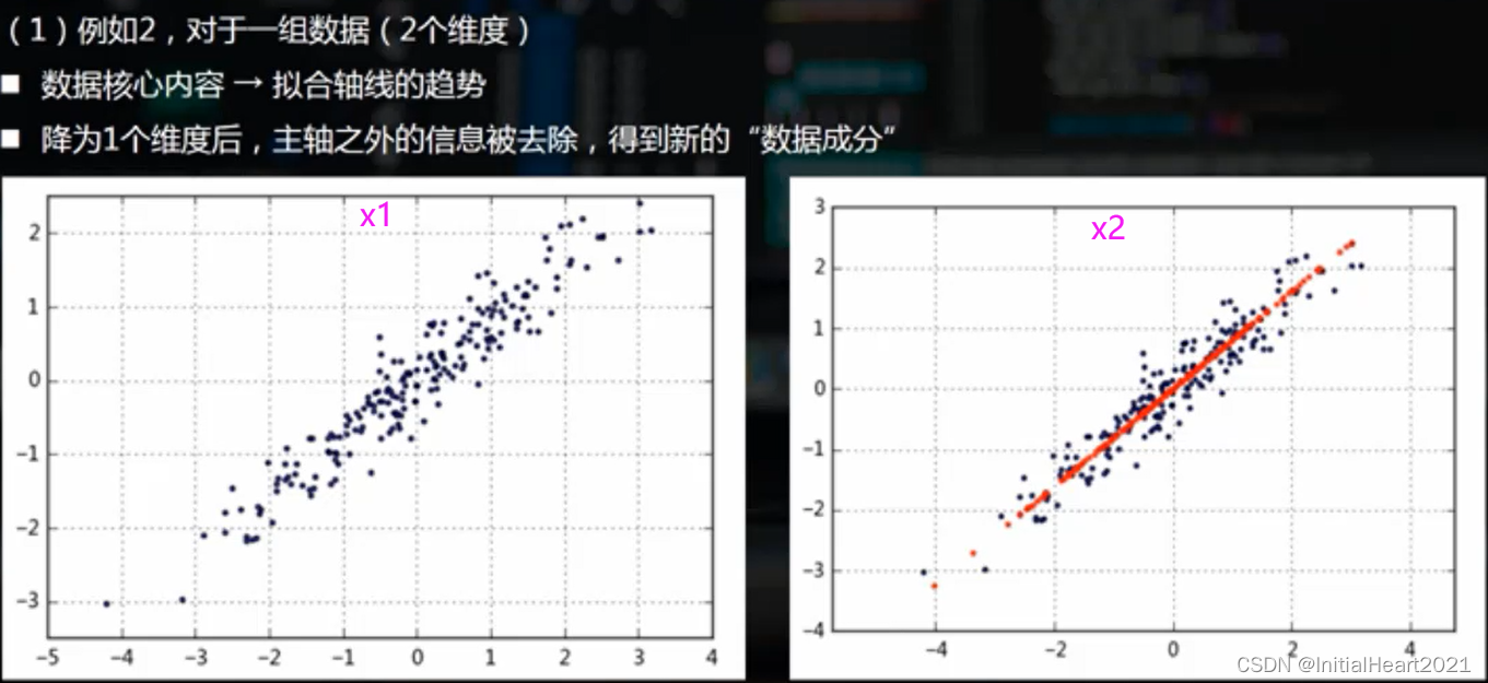
1.2.1.1.3 降维
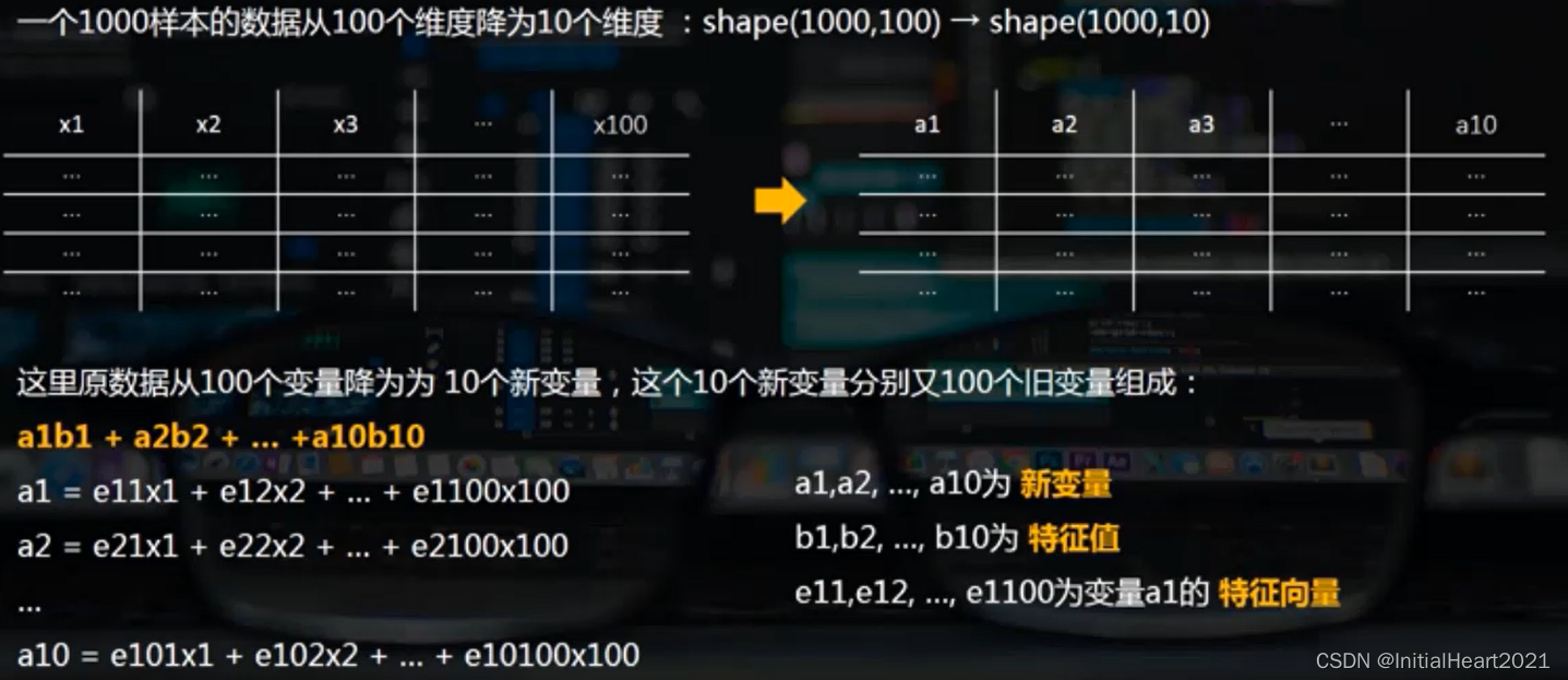
1.2.1.1.4 主成分的筛选
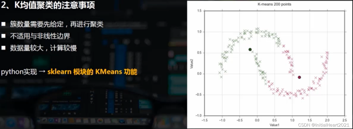
- 降维
- 主成分
- 累计贡献率

1.2.1.1.4 主成分的含义及用法

1.3 K-means聚类

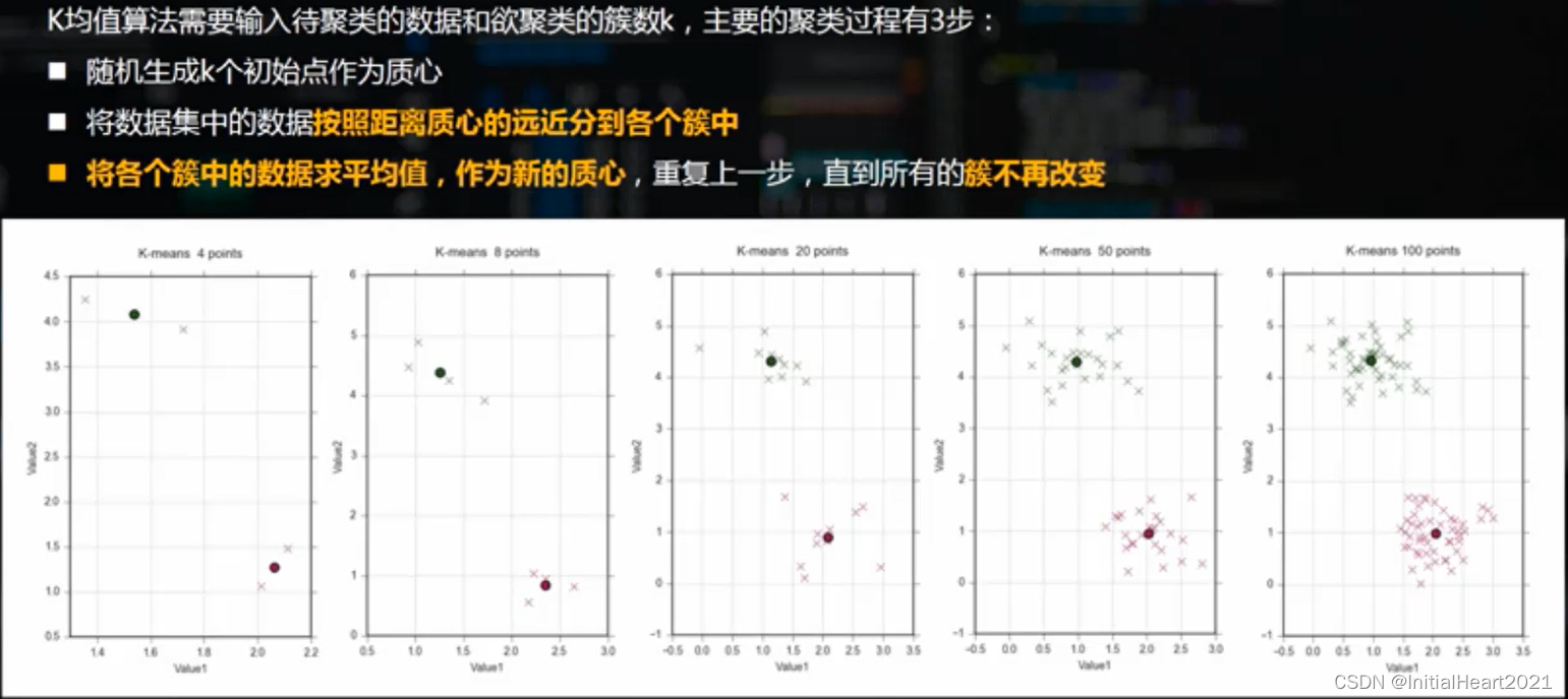
1.3.1 K均值算法实现逻辑
1.3.2 K均值聚类的注意事项
二、代码实现
2.1 PCA主成分分析
- 最广泛无监督算法 + 基础的降维算法
- PCA(Principal Component Analysis)是一种常用的数据分析方法。PCA通过线性变换将原始数据变换为一组各维度线性无关的表示,可用于提取数据的主要特征分量,常用于高维数据的降维。
import numpy as np
import pandas as pd
import matplotlib.pyplot as plt
%matplotlib inline
# 步骤一(替换sans-serif字体)
plt.rcParams['font.sans-serif'] = ['SimHei']

# 步骤二(解决坐标轴负数的负号显示问题
plt.rcParams['axes.unicode_minus'] = False
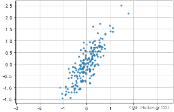
2.1.1 二维数据降维
# 创建数据

rng = np.random.RandomState(2)

# 矩阵相乘
data = np.dot(rng.rand(2,2), rng.randn(2, 200)).T
df = pd.DataFrame({
    'X1': data[:, 0],
    'X2': data[:, 1]
})

# 散点图
plt.scatter(df['X1'], df['X2'], alpha = 0.8, marker = '.')

# 坐标轴每个单位表示的刻度相同
plt.axis('equal')
plt.grid()
2.1.1.1 2 维 ——> 1 维
sklearn.decomposition.PCA(
	n_components=None,
	copy=True,
	whiten=False,
	svd_solver='auto',
	tol=0.0,
	iterated_power='auto',
	random_state=None,
)

n_components:PCA 算法中所要保留的主成分个数 n,即保留下来的特征个数

copy:True or False,表示是否在运行算法时,将原始训练数据赋值一份

fit(X, y=None):调用 fit方法的对象本身,如:pca.fit(X),表示用 X 对pca这个对象进行训练
# 二维数据降维:构建模型,主成分分析

# 加载主成分分析模型 PCA
from sklearn.decomposition import PCA

# 降为 1维
pca = PCA(n_components = 1)

# 构建模型
pca.fit(df)
运行结果

PCA(copy=True, iterated_power='auto', n_components=1, random_state=None,svd_solver='auto', tol=0.0, whiten=False)
# 特征值
print(pca.explained_variance_)

# 返回具有最大方差的成分,即特征向量
print(pca.components_)

# 0.68 * ((0.51 * x1) + (0.85 * x2))
运行结果

[0.67663501]

[[0.51517079 0.85708754]]
# 返回保留的成分个数
print(pca.n_components_)
print(pca.n_components)

# 结果降为几个维度,就有几个特征值;原始数据有几个维度,就有几个特征向量
print(pca.explained_variance_ratio_)
运行结果

1
1
[0.92716656]
# 这里是shape(200,2)降为shape(200,1),只有1个特征值,对应2个特征向量
# 降维后主成分 A1 = 0.52 * X1 + 0.86 * X2
# 成分的结果值 = 0.68 * (-0.77*x1 -0.62 * x2) #通过这个来筛选它的主成分


# 数据转换,将原始二维数据转换为降维后的一维数据
df_pca = pca.transform(df)

# 数据转换,将降维后的一维数据转换成原始的二维数据
df_inverse = pca.inverse_transform(df_pca)

print('original shape:', df.shape)
print('transformed shape:', df_pca.shape)
运行结果

original shape: (200, 2)
transformed shape: (200, 1)
# 原始数据
print(df.head(10))

# 降维数据
print(df_pca[:10])

# 反算数据
print(df_inverse[:10])
运行结果

         X1        X2
0 -0.759383 -0.607229
1 -0.395182 -0.935912
2  0.236474  0.565566
3 -0.523886 -0.364576
4 -0.488779 -1.043553
5 -0.399136 -0.546887
6  0.192457 -0.502409
7  1.007959  1.403810
8  0.009926 -0.114596
9 -0.522410 -1.202168
————————————————————————————————————————————————
[[-0.9337832 ]
 [-1.02786737]
 [ 0.58444096]
 [-0.60448782]
 [-1.16834379]
 [-0.69647639]
 [-0.35358286]
 [ 1.70033598]
 [-0.11522776]
 [-1.3216165 ]]
 ————————————————————————————————————————————————
[[-0.47335483 -0.77915224]
 [-0.52182425 -0.85979061]
 [ 0.30878991  0.52209877]
 [-0.30371147 -0.49691727]
 [-0.5941936  -0.98019121]
 [-0.3511013  -0.57575954]
 [-0.17445257 -0.28186976]
 [ 0.88366643  1.47851849]
 [-0.05165898 -0.07757857]
 [-0.67315522 -1.11155934]]
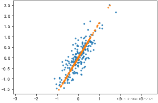
# 原始数据散点图
plt.scatter(df['X1'], df['X2'], alpha = 0.8, marker = '.')

# 转换之后的散点,红色的就是最后的特征数据
plt.scatter(df_inverse[:, 0], df_inverse[:, 1], alpha = 0.8, marker = '.')

plt.axis('equal')
2.1.2 多维数据降维
# 多维数据降维,使用自带的图像数据进行测试

from sklearn.datasets import load_digits

digits = load_digits()

print(type(digits))
print(digits.data[: 2])

# 总共1797条数据
print('数据长度为:%i 条' % len(digits['data']))

# 每条数据有 64 个变量
print('数据形状为:', digits['data'].shape)

print('字段:', digits.keys())

print('分类(数值):', digits.target)

print('分类(名称):', digits.target_names)
运行结果

<class 'sklearn.utils.Bunch'>

[[ 0.  0.  5. 13.  9.  1.  0.  0.  0.  0. 13. 15. 10. 15.  5.  0.  0.  3.
  15.  2.  0. 11.  8.  0.  0.  4. 12.  0.  0.  8.  8.  0.  0.  5.  8.  0.
   0.  9.  8.  0.  0.  4. 11.  0.  1. 12.  7.  0.  0.  2. 14.  5. 10. 12.
   0.  0.  0.  0.  6. 13. 10.  0.  0.  0.]
 [ 0.  0.  0. 12. 13.  5.  0.  0.  0.  0.  0. 11. 16.  9.  0.  0.  0.  0.
   3. 15. 16.  6.  0.  0.  0.  7. 15. 16. 16.  2.  0.  0.  0.  0.  1. 16.
  16.  3.  0.  0.  0.  0.  1. 16. 16.  6.  0.  0.  0.  0.  1. 16. 16.  6.
   0.  0.  0.  0.  0. 11. 16. 10.  0.  0.]]

数据长度为:1797 条

数据形状为: (1797, 64)

字段: dict_keys(['data', 'target', 'target_names', 'images', 'DESCR'])

分类(数值): [0 1 2 ... 8 9 8]

分类(名称): [0 1 2 3 4 5 6 7 8 9]
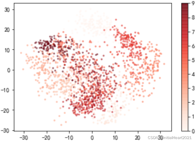
2.1.2.1 64维 ——> 2维
# 将上述数据由 64 维降为 2维,降维后的 2个维度肯定都是主成分

# 降为 2 维
pca = PCA(n_components = 2)

# 相当于先 fit 构建模型,再 transform 进行转换
projected = pca.fit_transform(digits['data'])

print('original shape:', digits['data'].shape)

print('transformed shape:', projected.shape)

# 2个 特征值
print('特征值:', pca.explained_variance_)

# 2个成分,每个成分都有64个特征向量
print('特征向量:', pca.components_.shape)
运行结果

original shape: (1797, 64)

transformed shape: (1797, 2)

特征值: [179.0069301  163.71774688]

特征向量: (2, 64)
plt.scatter(
    projected[:, 0],
    projected[:, 1],
    s = 10,
    c = digits.target,
    cmap = 'Reds',
    edgecolor = 'none',
    alpha = 0.6
)
plt.colorbar()
2.1.2.2 64维 ——> 10维
# 将上述数据降为10维,并求主要成分
from sklearn.datasets import load_digits
digits = load_digits()
# 降为10维
pca = PCA(n_components= 10)
# 相当于先 fit 构建模型,再 transform 进行转换
projecteds = pca.fit_transform(digits['data'])
print('original shape:', digits['data'].shape)
print('transformed shape:', projecteds.shape)
# 输出特征值 ;10个特征值
print(pca.explained_variance_)
# 输出特征向量形状
print(pca.components_.shape)
s = pca.explained_variance_
c_s = pd.DataFrame({
'x': s,
'x_cumsum': s.cumsum()/s.sum()
})
print(c_s)
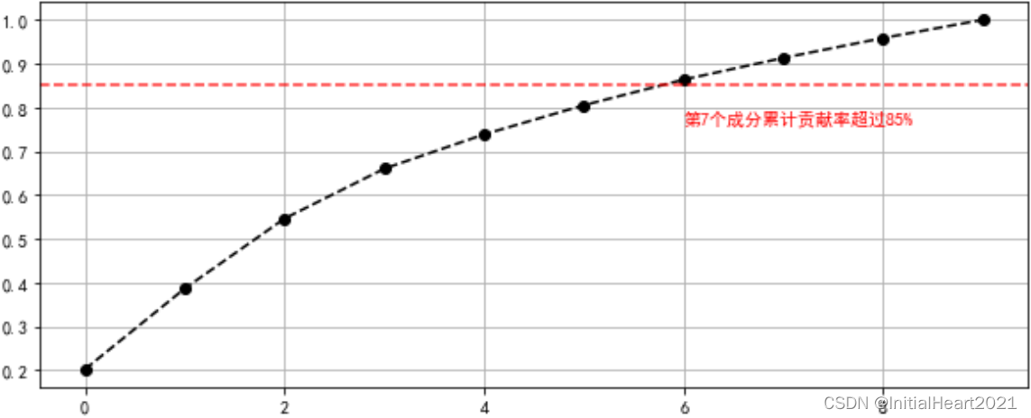
c_s['x_cumsum'].plot(style = '--ko', linestyle = '--', figsize = (10,4))
plt.axhline(0.85, color= 'r', linestyle = '--',alpha = 0.8)
plt.text(6, c_s['x_cumsum'].iloc[6]-0.1, '第7个成分累计贡献率超过85%', color = 'r')
plt.grid()
运行结果

original shape: (1797, 64)
transformed shape: (1797, 10)
[179.0069301  163.71774688 141.78843907 101.10037264  69.51316432
  59.10849447  51.88383863  44.01507618  40.30814729  37.01123765]
(10, 64)
            x  x_cumsum
0  179.006930  0.201709
1  163.717747  0.386189
2  141.788439  0.545959
3  101.100373  0.659881
4   69.513164  0.738210
5   59.108494  0.804814
6   51.883839  0.863278
7   44.015076  0.912875
8   40.308147  0.958295
9   37.011238  1.000000
2.1.3 K-means聚类
- K-means聚类是最常用的机器学习聚类算法,且为典型的基于距离的聚类算法。主要步骤为:
# 创建模型
kmeans = KMeans(n_clusters=4)

# 导入数据
kmeans.fit(x)

# 预测每个数据属于哪个类
y_kmeans = kmeans.predict(x)

# 每个类的中心点
centroids = kmeans.cluster_centers_
1.先使用 sklearn 自带的生成器生成数据
make_blobs(
    n_samples=100,
    n_features=2,
    centers=3,
    cluster_std=1.0,
    center_box=(-10.0, 10.0),
    shuffle=True,
    random_state=None,
)

n_samples:生成的样本总数
centers:类别数
cluster_std:每个类别的方差,如果多类数据不同方差可设置为[std1,std2,...stdn]
random_state:随机数种子
x 生成的数据
y 数据对应的类别
n_features:每个样本的特征数
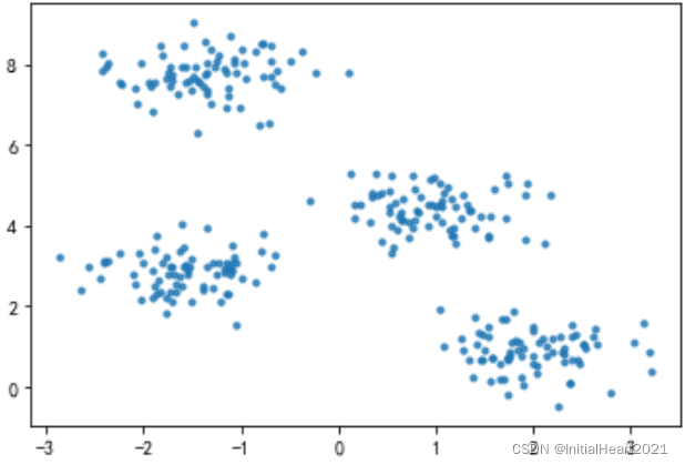
# make_blobs聚类数据生成器
from sklearn.datasets.samples_generator import make_blobs

x, y_true = make_blobs(
	n_samples=300,     # 生成300条数据
	centers=4,         # 四类数据
	cluster_std=0.5,   # 方差一致
	random_state = 0
)

plt.scatter(x[:, 0], x[:, 1], s = 10, alpha = 0.8)
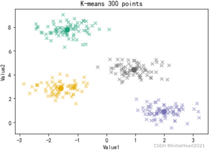
# 通过sklearn的 KMeans 进行聚类分析

from sklearn.cluster import KMeans

# 创建模型
kmeans = KMeans(n_clusters=4)

# 导入数据
kmeans.fit(x)

# 预测每个数据属于哪个类
y_kmeans = kmeans.predict(x)

# 每个类的中心点
centroids = kmeans.cluster_centers_

plt.scatter(x[:, 0], x[:, 1], s = 30, c = y_kmeans, cmap='Dark2', alpha = 0.5, marker='x')

plt.scatter(centroids[:, 0], centroids[:, 1], s = 70, c = [0,1,2,3], cmap = 'Dark2', marker = 'o')

plt.title('K-means 300 points')

plt.xlabel('Value1')

plt.ylabel('Value2')
版权声明:本文为博主原创文章,未经博主允许不得转载。


 被折叠的 条评论
为什么被折叠?
被折叠的 条评论
为什么被折叠?
 到【灌水乐园】发言


