Paper Notes: Graph Convolutional Neural Networks for Web-Scale Recommender Systemste

Graph Convolutional Neural Networks for Web-Scale Recommender Systems

• LINK: https://arxiv.org/abs/1806.01973

• CLASSIFICATION: RECOMMENDER-SYSTEM, GCN

• YEAR: Submitted on 6 Jun 2018

• FROM: KDD 2018

• WHAT PROBLEM TO SOLVE: The main challenge is to scale both the training as well as inference of GCN-based node embeddings to graphs with billions of nodes and tens of billions of edges. Scaling up GCNs is difficult because many of the core assumptions underlying their design are violated when working in a big data environment.

• SOLUTION: We develop a data-efficient Graph Convolutional Network (GCN) algorithm PinSage, which combines efficient random walks and graph convolutions to generate embeddings of nodes (i.e., items) that incorporate both graph structure as well as node feature information.

• CORE POINT:

  • Key insights to drastically improve the scalability of GCNs

    • On-the-fly convolutions

      PinSage algorithm performs efficient, localized convolutions by sampling the neighborhood around a node and dynamically constructing a computation graph from this sampled neighborhood.

    • Producer-consumer minibatch construction

      A large-memory, CPU-bound producer efficiently samples node network neighborhoods and fetches the necessary features to define local convolutions, while a GPU-bound TensorFlow model consumes these pre-defined computation graphs to efficiently run stochastic gradient decent.

    • Efficient MapReduce inference

      Given a fully-trained GCN model, we design an efficient MapReduce pipeline that can distribute the trained model to generate embeddings for billions of nodes, while minimizing repeated computations.

  • New training techniques and algorithmic innovations

    • Constructing convolutions via random walks

      Random sampling is suboptimal, and we develop a new technique using short random walks to sample the computation graph. An additional benefit is that each node now has an importance score, which we use in the pooling/aggregation step.

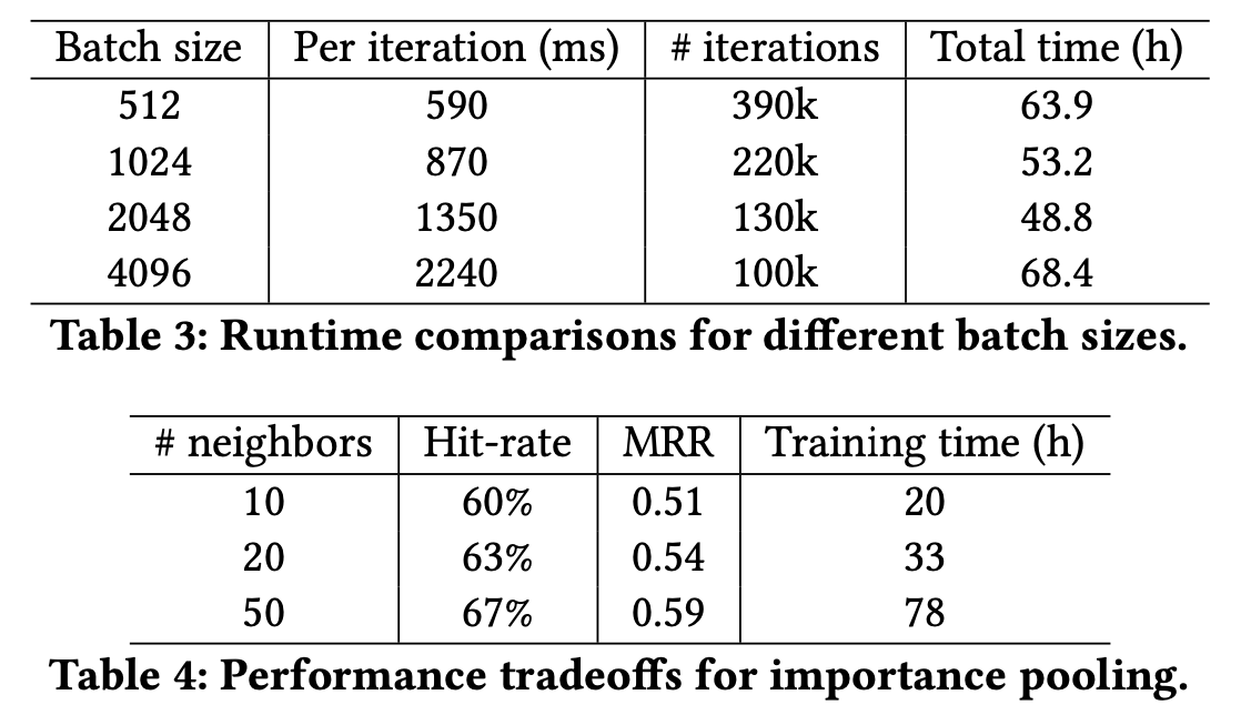
    • Importance pooling

      We introduce a method to weigh the importance of node features in this aggregation based upon random-walk similarity measures.

    • Curriculum training

      The algorithm is fed harder-and-harder examples during training.

  • Difference between GraphSage and PinSage

    We fundamentally improve upon GraphSAGE by removing the limitation that the whole graph be stored in GPU memory, using low-latency random walks to sample graph neighborhoods in a producer-consumer architecture.

  • Model Architecture

    Our task is to generate high-quality embeddings or representations of pins that can be used for recommendation (e.g., via nearest-neighbor lookup for related pin recommendation, or for use in a downstream re-ranking system).

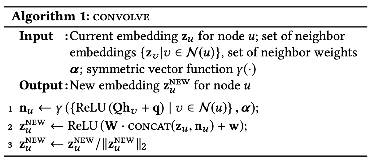
    • Forward propagation algorithm

      The normalization in Line 3 makes training more stable, and it is more efficient to perform approximate nearest neighbor search for normalized embeddings.

      

    • Importance-based neighborhoods

      In PinSage we define importance-based neighborhoods, where the neighborhood of a node u is defined as the T nodes that exert the most influence on node u. Concretely, we simulate random walks starting from node u and compute the L1-normalized visit count of nodes visited by the random walk. The neighborhood of u is then defined as the top T nodes with the highest normalized visit counts with respect to node u.

      In particular, we implement γ in Algorithm 1 as a weighted-mean, with weights defined according to the L1 normalized visit counts. We refer to this new approach as importance pooling.

    • Stacking convolutions

      We use multiple layers of convolutions, where the inputs to the convolutions at layer k depend on the representations output from layer k − 1 (Figure 1) and where the initial (i.e., “layer 0”) representations are equal to the input node features. Note that the model parameters in Algorithm 1 (Q, q, W, and w) are shared across the nodes but differ between layers.

      

  • Model Training

    • Loss function

      

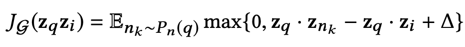
      $P_n(q)$ denotes the distribution of negative examples for item q, and ∆ denotes the margin hyper-parameter.

    • Multi-GPU training with large minibatches

      With multiple GPUs, we first divide each minibatch (Figure 1 bottom) into equal-sized portions. Each GPU takes one portion of the minibatch and performs the computations using the same set of parameters. After backward propagation, the gradients for each parameter across all GPUs are aggregated together, and a single step of synchronous SGD is performed.

      We use a gradual warmup procedure that increases learning rate from small to a peak value in the first epoch according to the linear scaling rule. Afterwards the learning rate is decreased exponentially.

    • Producer-consumer minibatch construction

      We use a re-indexing technique to create a sub-graph G′= (V′, E′) containing nodes and their neighborhood, which will be involved in the computation of the current minibatch. A small feature matrix containing only node features relevant to computation of the current minibatch is also extracted such that the order is consistent with the index of nodes in G′.

      We design a producer-consumer pattern to run GPU computation at the current iteration and CPU computation at the next iteration in parallel.

    • Sampling negative items

      To improve efficiency when training with large batch sizes, we sample a set of 500 negative items to be shared by all training examples in each minibatch.

      The inner product of the positive example (pair of items (q,i)) is larger than that of the q and each of the 500 negative items is too “easy” and does not provide fine enough “resolution” for the system to learn. To solve the above problem, for each positive training example (i.e., item pair (q,i)), we add “hard” negative examples, i.e., items that are somewhat related to the query item q, but not as related as the positive item i.

      Items ranked at 2000-5000 are randomly sampled as hard negative items. As illustrated in Figure 2, the hard negative examples are more similar to the query than random negative examples, and are thus challenging for the model to rank, forcing the model to learn to distinguish items at a finer granularity.

      • Curriculum training scheme

        In the first epoch of training, no hard negative items are used, so that the algorithm quickly finds an area in the parameter space where the loss is relatively small. We then add hard negative items in subsequent epochs, focusing the model to learn how to distinguish highly related pins from only slightly related ones. At epoch n of the training, we add n − 1 hard negative items to the set of negative items for each item.

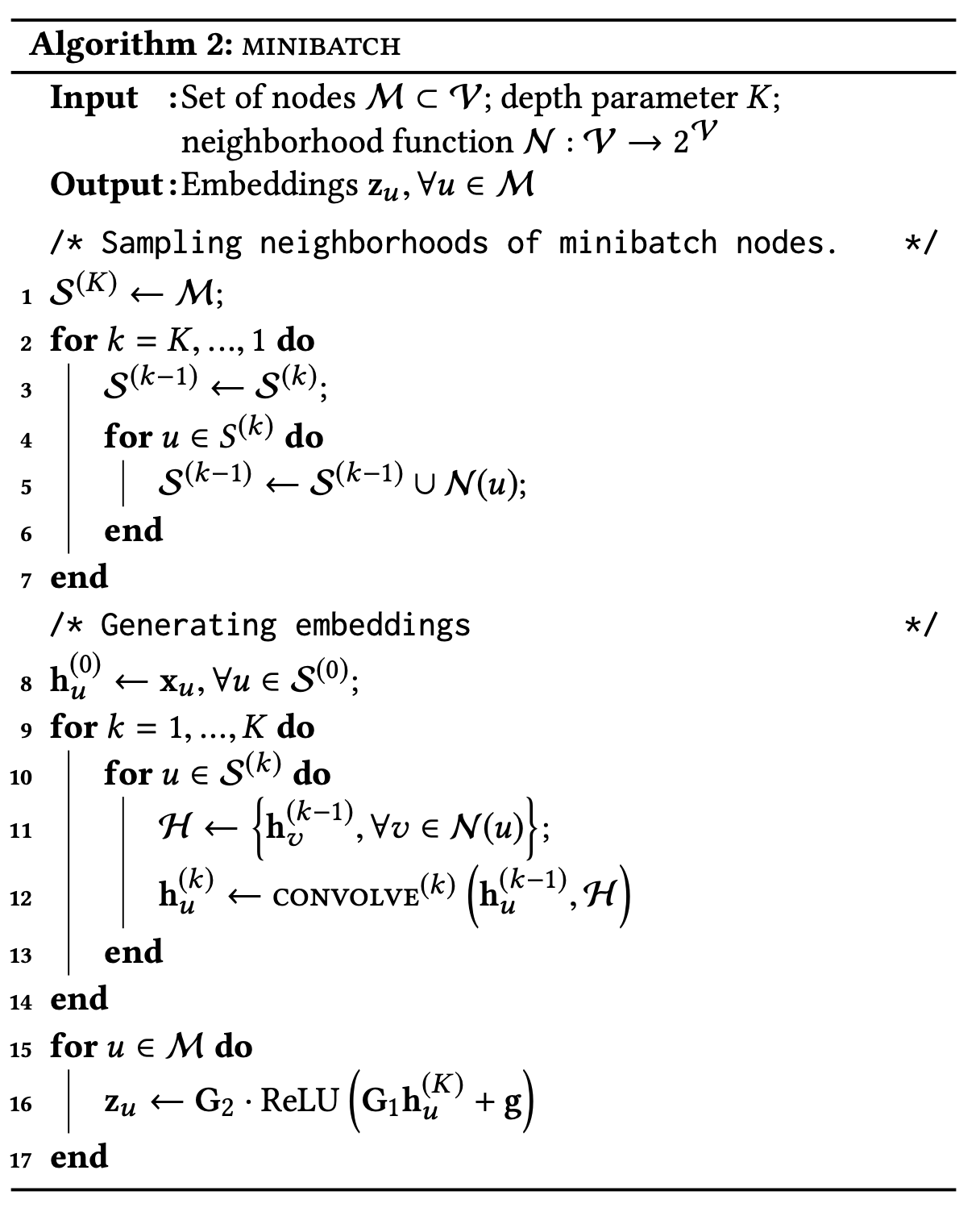
  • Node Embeddings via MapReduce

    Naively computing embeddings for nodes using Algorithm 2 leads to repeated computations caused by the overlap between K-hop neighborhoods of nodes.

    To ensure efficient inference, we develop a MapReduce approach that runs model inference without repeated computations. We observe that inference of node embeddings very nicely lends itself to MapReduce computational model.

  

  The MapReduce pipeline has two key parts:

  1. One MapReduce job is used to project all pins to a low-dimensional latent space, where the aggregation operation will be performed (Algorithm 1, Line 1).
  2. Another MapReduce job is then used to join the resulting pin representations with the ids of the boards they occur in, and the board embedding is computed by pooling the features of its (sampled) neighbors.

  • Experimental

    We evaluate the embeddings generated by PinSage in two tasks: recommending related pins and recommending pins in a user’s home/news feed.

    • Features used for learning

      To generate feature representation xq for each pin q, we concatenate visual embeddings (4,096 dimensions), textual annotation embeddings (256 dimensions), and the log degree of the node/pin in the graph.

    • Baselines for comparison

      1. Visual embeddings (Visual): Uses nearest neighbors of deep visual embeddings for
      2. Annotation embeddings (Annotation): Recommends based on nearest neighbors in terms of annotation embeddings.
      3. Combined embeddings (Combined): Recommends based on concatenating visual and annotation embeddings, and using a 2-layer multi-layer perceptron to compute embeddings that capture both visual and annotation features.
      4. Graph-based method (Pixie): This random-walk-based method uses biased random walks to generate ranking scores by simulating random walks starting at query pin q. Items with top K scores are retrieved as recommendations.

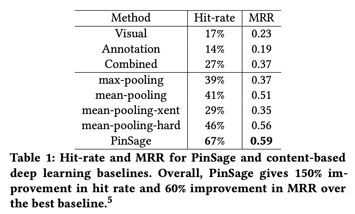
    • Offline Evaluation

      Define the hit-rate as the fraction of queries q where i was ranked among the top K of the test sample (i.e., where i ∈ NNq ). This metric directly measures the probability that recommendations made by the algorithm contain the items related to the query pin q. In our experiments K is set to be 500.

      

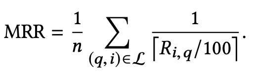
      Mean Reciprocal Rank (MRR), which takes into account of the rank of the item j among recommended items for query item q. The scaling factor 100 ensures that, for example, the difference between rank at 1, 000 and rank at 2, 000 is still noticeable, instead of being very close to 0.

      

      • Embedding similarity distribution

        Another indication of the effectiveness of the learned embeddings is that the distances between random pairs of item embeddings are widely distributed.

        

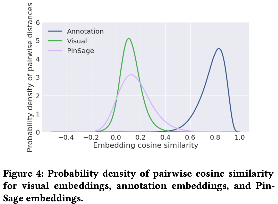
        Another important advantage of having such a wide-spread in the embeddings is that it reduces the collision probability of the subsequent LSH algorithm, thus increasing the efficiency of serving the nearest neighbor pins during recommendation.

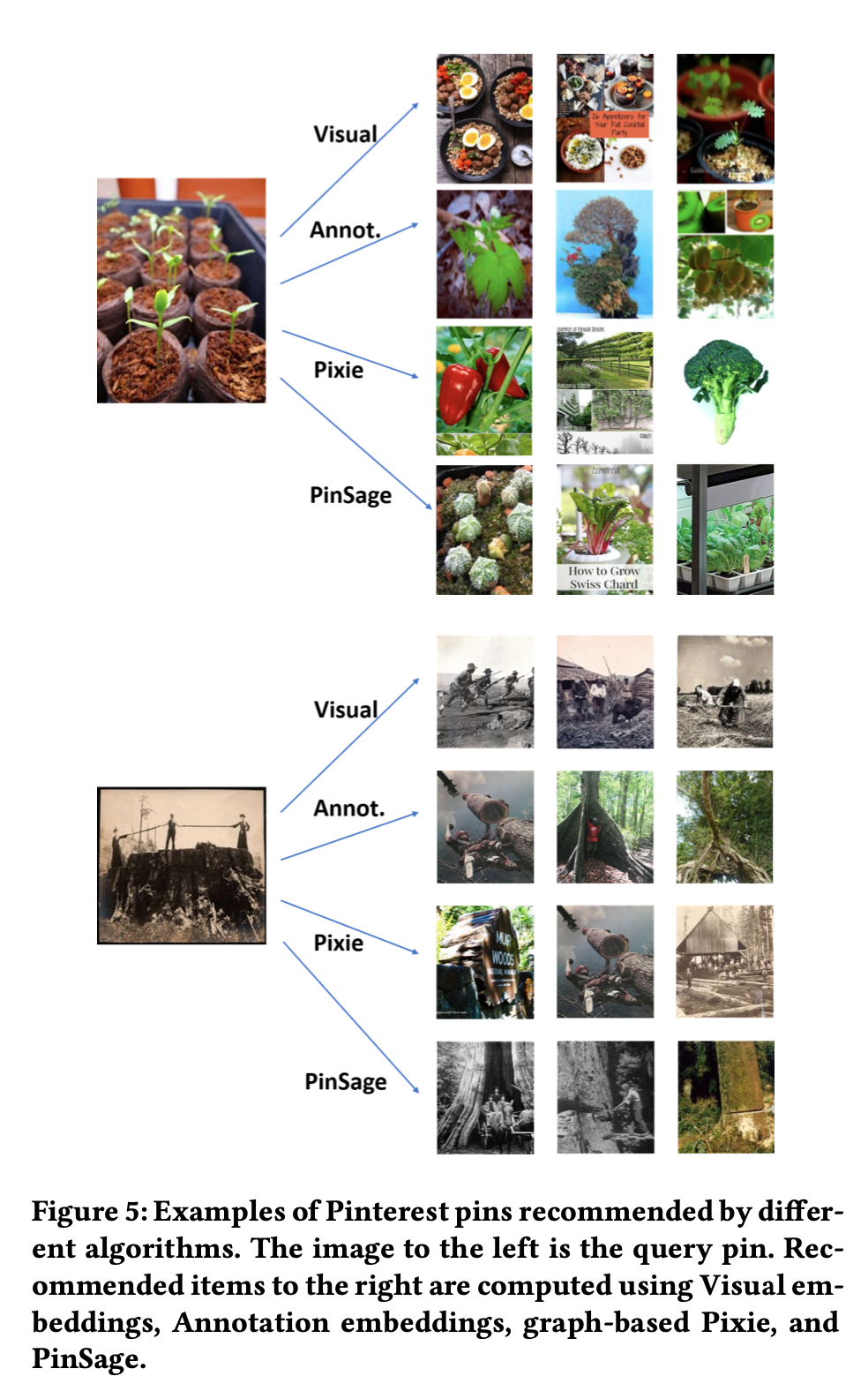
    • User Studies

      In the user study, a user is presented with an image of the query pin, together with two pins retrieved by two different recommendation algorithms. The user is then asked to choose which of the two candidate pins is more related to the query pin. Users are instructed to find various correlations between the recommended items and the query item, in aspects such as visual appearance, object category and personal identity.

      

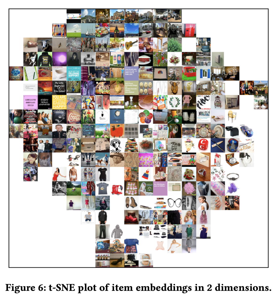
      2D t-SNE coordinates:

      

    • Production A/B Test

    • Training and Inference Runtime Analysis

      One advantage of GCNs is that they can be made inductive: at the inference (i.e., embedding generation) step, we are able to compute embeddings for items that were not in the training set. This allows us to train on a subgraph to obtain model parameters, and then make embed nodes that have not been observed during training. Also note that it is easy to compute embeddings of new nodes that get added into the graph over time. This means that recommendations can be made on the full (and constantly growing) graph.

      

• EXISTING PROBLEMS: No public data, no public code.

• IMPROVEMENT IDEAS: 404