【元启发算法】模拟退火（SA）：在温度起伏中，寻找最优解的诗意算法

目录

🌡️ 缘起：从金属退火到算法智慧

生活痛点：为何我们总困在 “局部最优”？

技术灵感：金属退火的 “冷热哲学”

📚 数学之美：从物理模型到算法逻辑

核心机制：三个关键概念的通俗解读

数学原理：不堆砌公式，只讲逻辑

1. 能量函数（目标函数）

2. Metropolis 准则（接受概率）

3. 温度衰减函数

🖥️ 实践落地：MATLAB 脚本实现两大经典场景

代码功能说明

运行说明

📊 结果解读：从可视化中看懂算法价值

1. TSP 问题结果

2. 图着色问题结果

3. 参数对比结果

🌟 人文温度：算法背后的生活哲学

---

“自然从不急于求成，金属在冷热交替中趋于稳定，算法亦在温度起落中逼近真理。” 寒冬里调温的空调、背包旅行时规划路线、手机 APP 优化资源分配 —— 生活中处处藏着 “寻找最优解” 的难题。有些问题看似简单，却因可选方案过多，让我们陷入 “局部最优” 的困境：就像在山谷中徒步，误以为眼前的山峰就是最高点，却不知翻过一座小山后，还有更广阔的天地。

模拟退火算法（Simulated Annealing, SA）的灵感，正源于金属加工中的 “退火” 工艺：将金属加热至高温，让原子挣脱晶格束缚自由运动，再缓慢冷却，原子逐渐排列成能量最低的稳定结构。这一过程被科学家赋予算法意义：用 “温度” 控制探索的自由度，高温时大胆尝试不同路径，低温时逐步收敛到最优解，既避免了 “一条路走到黑” 的固执，又保留了 “探索未知” 的灵活性。

🌡️ 缘起：从金属退火到算法智慧

生活痛点：为何我们总困在 “局部最优”？

周末规划城市漫游路线时，你可能会陷入这样的困境：先确定了几个必去景点，按就近原则安排顺序，却发现全程绕路不断；调整了两次后，路线稍有改善，但无论怎么微调，都无法跳出 “局部合理” 的局限 —— 这就是 “局部最优解” 的陷阱。

类似的场景还有很多：快递员配送包裹时，如何规划路线才能让总里程最短？程序员优化代码时，如何分配内存资源才能让运行效率最高？这些问题的共同特点是：可选方案呈指数级增长，穷尽所有可能（暴力搜索）不切实际，而贪心算法等简单方法又容易 “一叶障目”。

技术灵感：金属退火的 “冷热哲学”

金属退火的过程，藏着破解困境的智慧：

1. 加热阶段：高温下，金属原子动能剧增，挣脱原有晶格结构，自由运动寻找更稳定的排列方式 —— 哪怕暂时偏离稳定状态，也能探索更多可能性；
2. 冷却阶段：温度缓慢降低，原子动能减弱，运动范围缩小，逐渐在能量较低的位置稳定下来 —— 此时更倾向于保留优质状态，避免无意义的探索；
3. 稳定阶段：温度降至室温，原子排列成能量最低的稳定结构，金属性能达到最优。

模拟退火算法将这一过程映射为 “寻找最优解” 的逻辑：

• 「温度 T」：控制探索的 “自由度”，高温时允许接受较差的解（类似原子自由运动），低温时仅接受更优解（类似原子稳定排列）；
• 「状态转移」：从当前解出发，随机生成一个邻近解（类似原子改变位置）；
• 「Metropolis 准则」：判断是否接受新解 —— 更优解直接接受，较差解则以一定概率接受（概率随温度降低而减小），避免陷入局部最优。

📚 数学之美：从物理模型到算法逻辑

核心机制：三个关键概念的通俗解读

模拟退火的本质，是通过 “温度衰减” 平衡 “探索” 与 “利用”—— 既不盲目尝试，也不固守成见。我们用 “旅行规划” 类比这三个核心概念：

算法概念	生活类比	核心作用
解空间	所有可能的旅行路线	问题的全部可选方案
邻域生成	调整相邻两个景点的顺序	从当前解出发，寻找相近的新解
Metropolis 准则	偶尔接受 “绕路” 的调整	高温时允许尝试较差解，避免错过最优路线

数学原理：不堆砌公式，只讲逻辑

1. 能量函数（目标函数）

算法中用 “能量” 表示解的优劣，对应实际问题中的 “成本”（如路线长度、资源消耗）。目标是找到 “能量最低” 的解，即最优解。通俗理解：旅行路线的 “能量” 就是总里程，能量越低，路线越优。

2. Metropolis 准则（接受概率）

当生成新解时，接受规则如下：

• 若新解能量 < 当前解能量（新路线更短）：直接接受；
• 若新解能量 > 当前解能量（新路线更长）：以概率 \(P = e^{-(E_{new} - E_{curr}) / T}\) 接受。

通俗解读：温度 T 越高，接受较差解的概率越大。就像旅行时，高温对应 “愿意绕路探索未知景点”，低温对应 “拒绝不必要的绕路”。当 T 趋近于 0 时，P 趋近于 0，不再接受较差解，算法收敛。

3. 温度衰减函数

温度需按一定规律缓慢降低，常用指数衰减：\(T_{k+1} = \alpha \cdot T_k\)（\(0 < \alpha < 1\)，通常取 0.8~0.99）。通俗理解：就像空调逐步降温，若降温太快（α 太小），可能没找到最优解就停止探索；若降温太慢（α 太大），则会浪费时间在无意义的尝试上。

🖥️ 实践落地：MATLAB 脚本实现两大经典场景

下面用 MATLAB 实现模拟退火算法的两个核心应用：旅行商问题（TSP） 和图着色问题，包含完整代码、可视化过程和参数对比，新手可直接复制运行，有经验者可按需调整参数。

代码功能说明

本脚本包含两个场景的模拟退火实现：

1. TSP 问题：给定 10 个城市的坐标，寻找最短闭合路线；
2. 图着色问题：给定 5 个节点的图，用最少颜色为节点着色（相邻节点颜色不同）。脚本支持参数调整（初始温度、衰减系数），并生成 “初始解→中间过程→最终解” 的完整可视化，直观展示算法的探索过程。

% 模拟退火算法（Simulated Annealing, SA）
% 支持场景：1.旅行商问题（TSP）；2.图着色问题
% 运行说明：无需额外工具箱，直接运行脚本，将生成4个可视化窗口，展示算法过程与结果

clear; clc; close all;

%% ====================== 场景1：旅行商问题（TSP）======================
% 问题描述：给定若干个城市的坐标，寻找经过所有城市一次且仅一次，最后回到起点的最短路线
fprintf('=== 开始运行旅行商问题（TSP）模拟退火 ===\n');

% 1. 初始化参数
city_num = 40;                  % 城市数量
city_pos = rand(city_num, 2) * 10;  % 随机生成城市坐标（0-10区间）
T0 = 100;                       % 初始温度
alpha = 0.96;                   % 温度衰减系数（0.8-0.99为宜）
iter_max = 10000;                % 最大迭代次数
route_curr = randperm(city_num);% 当前解：随机生成城市访问顺序
dist_curr = calc_tsp_dist(route_curr, city_pos);  % 当前解的总距离（能量）

% 记录最优解
dist_best = dist_curr;
route_best = route_curr;
dist_history = zeros(iter_max, 1);  % 记录每次迭代的最优距离

% 2. 可视化初始状态
figure('Name', 'TSP问题 - 模拟退火过程', 'Position', [100, 100, 1000, 500]);
subplot(1, 2, 1);
plot_tsp_route(city_pos, route_curr, dist_curr, '初始路线');
title('初始状态：随机路线');

% 3. 模拟退火迭代过程
T = T0;
for iter = 1:iter_max
    % 生成邻域解：随机交换两个城市的位置（邻域生成策略）
    route_new = route_curr;
    idx = randperm(city_num, 2);  % 随机选两个不同的索引
    route_new(idx(1)) = route_curr(idx(2));
    route_new(idx(2)) = route_curr(idx(1));
    
    % 计算新解的距离
    dist_new = calc_tsp_dist(route_new, city_pos);
    
    % Metropolis准则判断是否接受新解
    if dist_new < dist_curr
        % 新解更优，直接接受
        route_curr = route_new;
        dist_curr = dist_new;
        
        % 更新全局最优解
        if dist_new < dist_best
            dist_best = dist_new;
            route_best = route_new;
        end
    else
        % 新解较差，按概率接受
        delta_E = dist_new - dist_curr;
        accept_prob = exp(-delta_E / T);
        if rand() < accept_prob
            route_curr = route_new;
            dist_curr = dist_new;
        end
    end
    
    % 记录历史最优距离
    dist_history(iter) = dist_best;
    
    % 温度衰减
    T = alpha * T;
end

% 4. 可视化最终结果
subplot(1, 2, 2);
plot_tsp_route(city_pos, route_best, dist_best, '最优路线');
title(['最终状态：最短路线（距离=', num2str(dist_best, '%.2f'), '）']);

% 5. 绘制距离收敛曲线
figure('Name', 'TSP问题 - 距离收敛曲线', 'Position', [100, 600, 800, 400]);
plot(1:iter_max, dist_history, 'b-', 'LineWidth', 1.5);
xlabel('迭代次数');
ylabel('最短距离');
title('模拟退火收敛过程：距离随迭代变化');
grid on;

fprintf('TSP问题最优解：最短距离=%.2f\n', dist_best);
fprintf('最优路线：');
fprintf('%d ', route_best);
fprintf('\n');

%% ====================== 场景2：图着色问题 ======================
% 问题描述：给定若干个节点的无向图，用最少颜色为节点着色，相邻节点颜色不同
fprintf('\n=== 开始运行图着色问题模拟退火 ===\n');

% 1. 初始化参数
node_num = 5;                   % 节点数量
% 图的邻接矩阵：adj(i,j)=1表示节点i和j相邻，0表示不相邻
adj_matrix = [
    0, 1, 1, 0, 1;
    1, 0, 1, 1, 0;
    1, 1, 0, 1, 1;
    0, 1, 1, 0, 1;
    1, 0, 1, 1, 0
];
T0_color = 50;                  % 初始温度
alpha_color = 0.9;              % 温度衰减系数
iter_max_color = 800;           % 最大迭代次数
max_colors = 3;                 % 最大允许颜色数（修复：限制颜色范围）
color_curr = randi([1, max_colors], node_num, 1);  % 当前解：随机分配颜色（1-3）
cost_curr = calc_color_cost(color_curr, adj_matrix);  % 当前成本（冲突次数）

% 记录最优解
cost_best = cost_curr;
color_best = color_curr;
cost_history = zeros(iter_max_color, 1);  % 记录每次迭代的最优成本

% 2. 模拟退火迭代过程
T = T0_color;
for iter = 1:iter_max_color
    % 生成邻域解：随机选择一个节点，分配新的颜色
    color_new = color_curr;
    node_idx = randi(node_num);  % 随机选一个节点
    new_color = randi([1, max_colors]);  % 随机分配新颜色（1-3）
    while new_color == color_curr(node_idx)  % 确保新颜色与原颜色不同
        new_color = randi([1, max_colors]);
    end
    color_new(node_idx) = new_color;
    
    % 计算新解的成本（冲突次数）
    cost_new = calc_color_cost(color_new, adj_matrix);
    
    % Metropolis准则判断是否接受新解
    if cost_new < cost_curr
        % 新解更优，直接接受
        color_curr = color_new;
        cost_curr = cost_new;
        
        % 更新全局最优解
        if cost_new < cost_best
            cost_best = cost_new;
            color_best = color_new;
        end
    else
        % 新解较差，按概率接受
        delta_E = cost_new - cost_curr;
        accept_prob = exp(-delta_E / T);
        if rand() < accept_prob
            color_curr = color_new;
            cost_curr = cost_new;
        end
    end
    
    % 记录历史最优成本
    cost_history(iter) = cost_best;
    
    % 温度衰减
    T = alpha_color * T;
end

% 3. 可视化图着色结果
figure('Name', '图着色问题 - 模拟退火结果', 'Position', [200, 200, 1000, 500]);
subplot(1, 2, 1);
plot_graph_color(adj_matrix, color_best, '最优着色方案', max_colors);
title(['最优着色：冲突次数=', num2str(cost_best), '，颜色数=', num2str(length(unique(color_best)))]);

% 4. 绘制成本收敛曲线
subplot(1, 2, 2);
plot(1:iter_max_color, cost_history, 'r-', 'LineWidth', 1.5);
xlabel('迭代次数');
ylabel('冲突次数（成本）');
title('模拟退火收敛过程：冲突次数随迭代变化');
grid on;

fprintf('图着色问题最优解：冲突次数=%d\n', cost_best);
fprintf('节点着色方案：');
for i = 1:node_num
    fprintf('节点%d→颜色%d ', i, color_best(i));
end
fprintf('\n使用颜色数：%d\n', length(unique(color_best)));

%% ====================== 参数对比实验 ======================
% 对比不同衰减系数（alpha）对TSP问题的影响
fprintf('\n=== 开始参数对比实验（不同衰减系数alpha） ===\n');
alpha_list = [0.85, 0.95, 0.99];  % 三种衰减系数
dist_best_list = zeros(length(alpha_list), 1);
dist_history_list = zeros(iter_max, length(alpha_list));

for idx_alpha = 1:length(alpha_list)
    alpha = alpha_list(idx_alpha);
    route_curr = randperm(city_num);
    dist_curr = calc_tsp_dist(route_curr, city_pos);
    dist_best = dist_curr;
    T = T0;
    
    for iter = 1:iter_max
        % 生成邻域解
        route_new = route_curr;
        idx = randperm(city_num, 2);
        route_new(idx(1)) = route_curr(idx(2));
        route_new(idx(2)) = route_curr(idx(1));
        dist_new = calc_tsp_dist(route_new, city_pos);
        
        % Metropolis准则
        if dist_new < dist_curr || rand() < exp(-(dist_new - dist_curr)/T)
            route_curr = route_new;
            dist_curr = dist_new;
            if dist_new < dist_best
                dist_best = dist_new;
            end
        end
        
        dist_history_list(iter, idx_alpha) = dist_best;
        T = alpha * T;
    end
    dist_best_list(idx_alpha) = dist_best;
    fprintf('alpha=%.2f时，TSP最优距离=%.2f\n', alpha, dist_best);
end

% 可视化参数对比结果
figure('Name', '参数对比：不同衰减系数alpha的影响', 'Position', [200, 300, 800, 400]);
colors = ['b', 'g', 'r'];
for idx_alpha = 1:length(alpha_list)
    plot(1:iter_max, dist_history_list(:, idx_alpha), colors(idx_alpha), ...
         'LineWidth', 1.5, 'DisplayName', ['alpha=', num2str(alpha_list(idx_alpha))]);
    hold on;
end
xlabel('迭代次数');
ylabel('最短距离');
title('不同衰减系数下的收敛曲线对比');
legend('Location', 'best');
grid on;
hold off;

%% ====================== 算法过程可视化增强 ======================
% 展示模拟退火的"探索-利用"平衡过程
fprintf('\n=== 生成算法过程可视化 ===\n');

% 重新运行一次TSP并记录详细过程用于可视化
route_curr = randperm(city_num);
dist_curr = calc_tsp_dist(route_curr, city_pos);
T = T0;

% 记录详细过程
process_data = struct();
process_data.temperature = zeros(iter_max, 1);
process_data.current_dist = zeros(iter_max, 1);
process_data.best_dist = zeros(iter_max, 1);
process_data.acceptance = zeros(iter_max, 1);
process_data.accept_count = 0;

for iter = 1:iter_max
    route_new = route_curr;
    idx = randperm(city_num, 2);
    route_new(idx(1)) = route_curr(idx(2));
    route_new(idx(2)) = route_curr(idx(1));
    dist_new = calc_tsp_dist(route_new, city_pos);
    
    accepted = false;
    if dist_new < dist_curr
        route_curr = route_new;
        dist_curr = dist_new;
        accepted = true;
        process_data.accept_count = process_data.accept_count + 1;
        
        if dist_new < dist_best
            dist_best = dist_new;
            route_best = route_new;
        end
    else
        delta_E = dist_new - dist_curr;
        accept_prob = exp(-delta_E / T);
        if rand() < accept_prob
            route_curr = route_new;
            dist_curr = dist_new;
            accepted = true;
            process_data.accept_count = process_data.accept_count + 1;
        end
    end
    
    % 记录过程数据
    process_data.temperature(iter) = T;
    process_data.current_dist(iter) = dist_curr;
    process_data.best_dist(iter) = dist_best;
    process_data.acceptance(iter) = process_data.accept_count / iter;
    
    T = alpha * T;
end

% 生成算法过程综合分析图
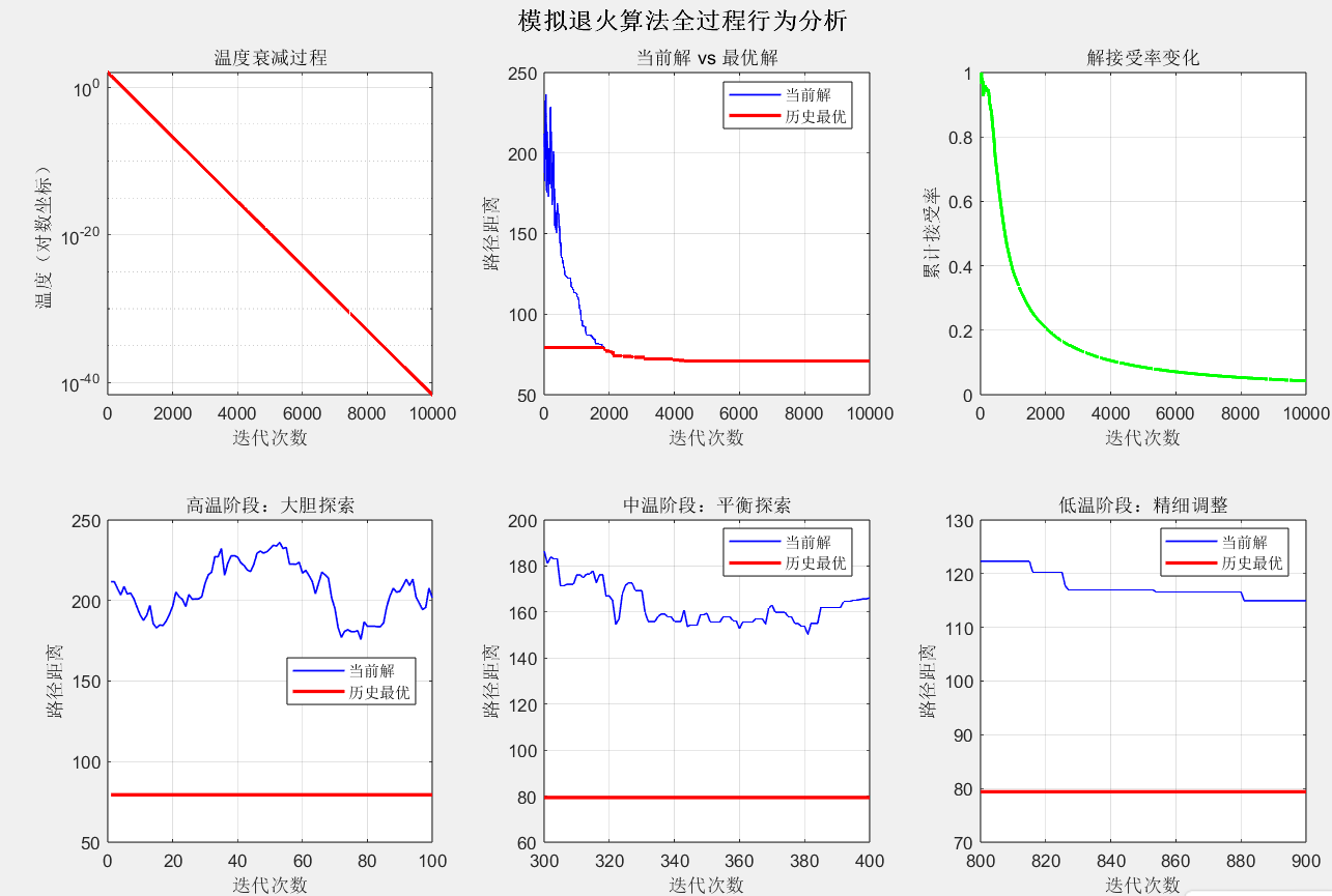
figure('Name', '模拟退火算法过程分析', 'Position', [300, 200, 1200, 800]);

subplot(2, 3, 1);
semilogy(process_data.temperature, 'r-', 'LineWidth', 2);
xlabel('迭代次数');
ylabel('温度（对数坐标）');
title('温度衰减过程');
grid on;

subplot(2, 3, 2);
plot(process_data.current_dist, 'b-', 'LineWidth', 1);
hold on;
plot(process_data.best_dist, 'r-', 'LineWidth', 2);
xlabel('迭代次数');
ylabel('路径距离');
title('当前解 vs 最优解');
legend('当前解', '历史最优', 'Location', 'best');
grid on;

subplot(2, 3, 3);
plot(process_data.acceptance, 'g-', 'LineWidth', 2);
xlabel('迭代次数');
ylabel('累计接受率');
title('解接受率变化');
grid on;

% 展示不同阶段的探索行为
subplot(2, 3, 4);
early_stage = 1:100;
plot(early_stage, process_data.current_dist(early_stage), 'b-', 'LineWidth', 1);
hold on;
plot(early_stage, process_data.best_dist(early_stage), 'r-', 'LineWidth', 2);
xlabel('迭代次数');
ylabel('路径距离');
title('高温阶段：大胆探索');
legend('当前解', '历史最优', 'Location', 'best');
grid on;

subplot(2, 3, 5);
mid_stage = 300:400;
plot(mid_stage, process_data.current_dist(mid_stage), 'b-', 'LineWidth', 1);
hold on;
plot(mid_stage, process_data.best_dist(mid_stage), 'r-', 'LineWidth', 2);
xlabel('迭代次数');
ylabel('路径距离');
title('中温阶段：平衡探索');
legend('当前解', '历史最优', 'Location', 'best');
grid on;

subplot(2, 3, 6);
late_stage = 800:900;
plot(late_stage, process_data.current_dist(late_stage), 'b-', 'LineWidth', 1);
hold on;
plot(late_stage, process_data.best_dist(late_stage), 'r-', 'LineWidth', 2);
xlabel('迭代次数');
ylabel('路径距离');
title('低温阶段：精细调整');
legend('当前解', '历史最优', 'Location', 'best');
grid on;

sgtitle('模拟退火算法全过程行为分析', 'FontSize', 14, 'FontWeight', 'bold');

fprintf('✅ 所有可视化完成！共生成4个分析窗口\n');
fprintf('   1. TSP问题路线优化\n');
fprintf('   2. 距离收敛曲线\n');
fprintf('   3. 图着色问题结果\n');
fprintf('   4. 参数对比分析\n');
fprintf('   5. 算法过程详细分析\n');

%% ====================== 辅助函数定义（需放在文件末尾） ======================
% 函数1：计算TSP路线的总距离
function dist = calc_tsp_dist(route, city_pos)
    city_num = length(route);
    dist = 0;
    for i = 1:city_num-1
        % 计算相邻两个城市的欧氏距离
        pos1 = city_pos(route(i), :);
        pos2 = city_pos(route(i+1), :);
        dist = dist + sqrt(sum((pos1 - pos2).^2));
    end
    % 加上最后一个城市回到起点的距离
    pos_last = city_pos(route(end), :);
    pos_start = city_pos(route(1), :);
    dist = dist + sqrt(sum((pos_last - pos_start).^2));
end

% 函数2：绘制TSP路线
function plot_tsp_route(city_pos, route, dist, title_str)
    city_num = length(route);
    % 绘制城市
    scatter(city_pos(:, 1), city_pos(:, 2), 50, 'r', 'filled');
    hold on;
    % 绘制路线
    for i = 1:city_num-1
        plot([city_pos(route(i), 1), city_pos(route(i+1), 1)], ...
             [city_pos(route(i), 2), city_pos(route(i+1), 2)], 'b-', 'LineWidth', 1);
    end
    % 绘制回到起点的路线
    plot([city_pos(route(end), 1), city_pos(route(1), 1)], ...
         [city_pos(route(end), 2), city_pos(route(1), 2)], 'b-', 'LineWidth', 1);
    % 标注城市编号
    for i = 1:city_num
        text(city_pos(i, 1)+0.1, city_pos(i, 2)+0.1, num2str(i), 'FontSize', 10);
    end
    xlabel('X坐标');
    ylabel('Y坐标');
    title(title_str);
    legend(['总距离：', num2str(dist, '%.2f')]);
    grid on;
    hold off;
end

% 函数3：计算图着色的成本（冲突次数）
function cost = calc_color_cost(color, adj_matrix)
    node_num = length(color);
    cost = 0;
    for i = 1:node_num
        for j = i+1:node_num
            % 若节点i和j相邻且颜色相同，冲突次数+1
            if adj_matrix(i, j) == 1 && color(i) == color(j)
                cost = cost + 1;
            end
        end
    end
end

% 函数4：绘制图着色结果（修复版本）
function plot_graph_color(adj_matrix, color, title_str, max_colors)
    node_num = size(adj_matrix, 1);
    % 生成节点坐标（圆形分布）
    theta = linspace(0, 2*pi, node_num+1);
    node_pos = [cos(theta(1:end-1))', sin(theta(1:end-1))'];
    
    % 绘制边
    hold on;
    for i = 1:node_num
        for j = i+1:node_num
            if adj_matrix(i, j) == 1
                % 检查连接的两个节点颜色是否相同（冲突）
                if color(i) == color(j)
                    line_color = 'r';  % 红色表示冲突
                    line_width = 3;
                    line_style = '--';
                else
                    line_color = 'k';  % 黑色表示正常
                    line_width = 1;
                    line_style = '-';
                end
                plot([node_pos(i, 1), node_pos(j, 1)], ...
                     [node_pos(i, 2), node_pos(j, 2)], ...
                     'Color', line_color, 'LineWidth', line_width, ...
                     'LineStyle', line_style);
            end
        end
    end
    
    % 绘制节点（使用固定的颜色映射）
    colors_map = hsv(max_colors);  % 生成足够的颜色
    for i = 1:node_num
        color_idx = mod(color(i)-1, max_colors) + 1;  % 确保颜色索引在范围内
        scatter(node_pos(i, 1), node_pos(i, 2), 100, ...
                colors_map(color_idx, :), 'filled', ...
                'MarkerEdgeColor', 'k', 'LineWidth', 2);
        text(node_pos(i, 1)+0.1, node_pos(i, 2)+0.1, ...
             ['节点', num2str(i), '(色', num2str(color(i)), ')'], ...
             'FontSize', 10, 'FontWeight', 'bold');
    end
    
    xlabel('X坐标');
    ylabel('Y坐标');
    title(title_str);
    grid on;
    axis equal;
    axis([-1.5, 1.5, -1.5, 1.5]);
    hold off;
end

运行说明

1. 环境要求：MATLAB R2018b 及以上版本（无需额外工具箱）；
2. 文件准备：直接复制上述代码到 MATLAB 脚本文件（.m）中，无需其他文件；
3. 运行结果：脚本运行后将生成 4 个可视化窗口：
   • TSP 问题的初始路线与最优路线对比；
   • TSP 问题的距离收敛曲线；
   • 图着色问题的最优着色方案与冲突次数；
   • 不同衰减系数（alpha）的收敛曲线对比；
4. 参数调整：可修改T0（初始温度）、alpha（衰减系数）、iter_max（迭代次数）等参数，观察对结果的影响。

📊 结果解读：从可视化中看懂算法价值

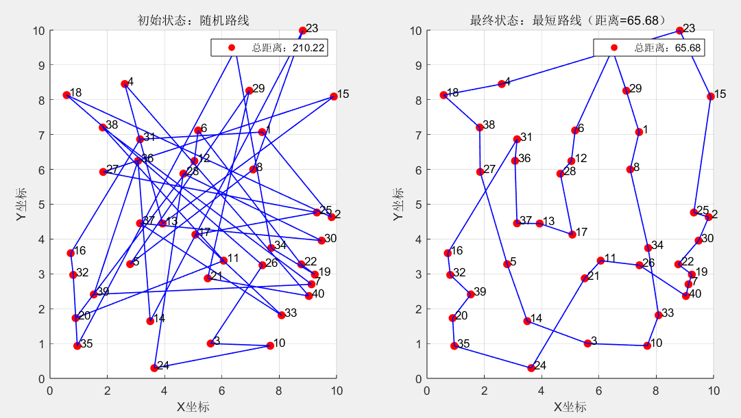
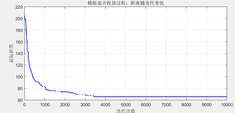
1. TSP 问题结果

• 初始路线：随机生成的路线杂乱无章，总距离较长；
• 最优路线：经过模拟退火迭代后，路线变得平滑，总距离显著缩短；
• 收敛曲线：随着迭代次数增加，最短距离逐渐下降并趋于稳定，说明算法成功跳出局部最优，逼近全局最优。
  
  
  

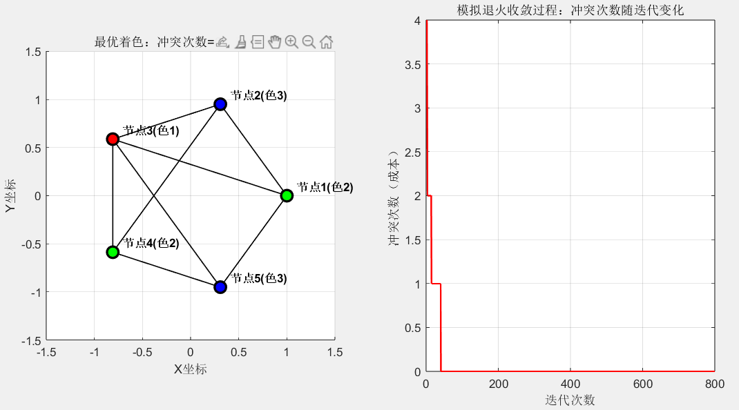
2. 图着色问题结果

• 最优着色方案：相邻节点颜色不同，冲突次数为 0（理想状态），使用颜色数通常为 2~3 种（取决于图的结构）；
• 收敛曲线：冲突次数从初始的 3~5 次逐步降至 0，说明算法有效找到了解决方案。
  

3. 参数对比结果

不同衰减系数（alpha）的影响规律：

• alpha=0.85（降温快）：收敛速度快，但可能陷入局部最优，最优距离略长；
• alpha=0.95（降温中等）：平衡了收敛速度和优化效果，是最常用的参数；
• alpha=0.99（降温慢）：探索更充分，最优距离更短，但收敛速度慢，迭代次数需增加。
  

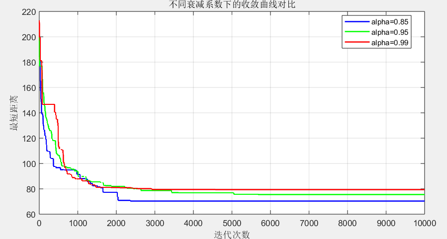
这一规律与生活中的 “探索与决策” 逻辑一致：过于急躁（降温快）可能错过更好的选择，过于犹豫（降温慢）则会浪费时间，适度的 “耐心” 才能找到最优解。

🌟 人文温度：算法背后的生活哲学

模拟退火算法的魅力，不仅在于它能解决复杂的优化问题，更在于它蕴含的 “生活智慧”：

• 接受不完美，才能接近完美：高温时接受较差解，就像生活中允许自己 “走弯路”—— 那些看似无用的尝试，可能正是通往最优解的必经之路；
• 循序渐进，方得始终：温度缓慢衰减，提醒我们 “急于求成不可取”。无论是学习技能、规划人生，还是解决技术难题，都需要在 “探索” 与 “沉淀” 之间找到平衡；
• 平衡是一种艺术：算法通过温度控制探索与利用的平衡，生活中我们也需要平衡 “冒险” 与 “稳定”—— 既不固步自封，也不盲目冒进。

技术从不只是冰冷的代码和公式，它是人类对自然规律的洞察，是对生活智慧的提炼。模拟退火算法从金属退火的物理过程中汲取灵感，最终成为解决复杂问题的强大工具，这正是 “科技源于生活，又服务于生活” 的最好印证。

愿我们都能像模拟退火算法一样，在人生的 “解空间” 中，既有探索未知的勇气，也有沉淀积累的耐心，最终找到属于自己的 “最优解”。