RNNs_gradients_vanishing

最新推荐文章于 2022-08-14 19:15:45 发布

Forlogen

最新推荐文章于 2022-08-14 19:15:45 发布

阅读量262

点赞数

CC 4.0 BY-SA版权

分类专栏： NLP

本文链接：https://blog.youkuaiyun.com/Forlogen/article/details/97304014

NLP 专栏收录该内容

64 篇文章

订阅专栏

本文通过对比Sigmoid和ReLU激活函数在简单循环神经网络中的表现，深入探讨了RNN中的梯度消失问题。实验结果显示，ReLU能有效避免梯度消失，提高模型学习效率。

摘要生成于 C知道，由 DeepSeek-R1 满血版支持，前往体验 >

内容来源于CS224n（2017）第七讲给出的示例代码，整理以便学习。

理解RNN中的梯度消失问题

本例将使用只有两层的简单的循环神经网络来了解下使用sigmoid和Relu的不同之处

# Setup
import numpy as np
import matplotlib.pyplot as plt

%matplotlib inline
plt.rcParams['figure.figsize'] = (10.0, 8.0) # set default size of plots
plt.rcParams['image.interpolation'] = 'nearest'
plt.rcParams['image.cmap'] = 'gray'

# for auto-reloading extenrnal modules
# see http://stackoverflow.com/questions/1907993/autoreload-of-modules-in-ipython
%load_ext autoreload
%autoreload 2

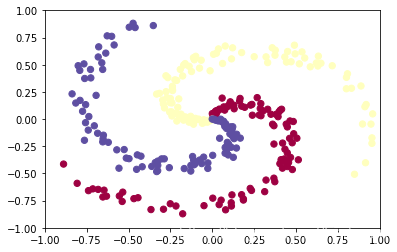
随机生成示例数据

#generate random data -- not linearly separable 
np.random.seed(0)
N = 100 # number of points per class
D = 2 # dimensionality
K = 3 # number of classes
X = np.zeros((N*K,D))
num_train_examples = X.shape[0]
y = np.zeros(N*K, dtype='uint8')
for j in range(K):
  ix = range(N*j,N*(j+1))
  r = np.linspace(0.0,1,N) # radius
  t = np.linspace(j*4,(j+1)*4,N) + np.random.randn(N)*0.2 # theta
  X[ix] = np.c_[r*np.sin(t), r*np.cos(t)]
  y[ix] = j
fig = plt.figure()
plt.scatter(X[:, 0], X[:, 1], c=y, s=40, cmap=plt.cm.Spectral)
plt.xlim([-1,1])
plt.ylim([-1,1])

OUTPUT: (-1, 1)

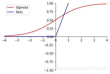
sigmoid 和relu

根据sigmoid函数图可以直观的看出，当输出靠近0或是1时，梯度会迅速的归于0，这时模型已无法从梯度中获得有用的信息，即发生了梯度消失问题。

而 $\max(0,x)$ ,并不会随着输入的增大而饱和，有效的避免了梯度消失的出现。

import math 
import numpy as np
import matplotlib.pyplot as plt
 
# set x's range
x = np.arange(-10,10,0.1)
 
y1=1/(1+math.e**(-x)) # sigmoid
y2=np.where(x<0,0,x) # relu
 
plt.xlim(-4,4)
plt.ylim(-1,1)
 
ax = plt.gca()
ax.spines['right'].set_color('none') 
ax.spines['top'].set_color('none')
ax.xaxis.set_ticks_position('bottom')   
ax.yaxis.set_ticks_position('left')
ax.spines['bottom'].set_position(('data', 0))
ax.spines['left'].set_position(('data', 0))
 
#Draw pic
plt.plot(x,y1,label='sigmoid',linestyle="-", color="red")
plt.plot(x,y2,label='relu',linestyle="-", color="blue")
 
# Title
plt.legend(['Sigmoid','Relu'])
plt.show()

OUTPUT:

def sigmoid(x):
    x = 1/(1+np.exp(-x))
    return x

def sigmoid_grad(x):
    return (x)*(1-x)

def relu(x):
    return np.maximum(0,x)

构建简单的循环神经网络

#function to train a three layer neural net with either RELU or sigmoid nonlinearity via vanilla grad descent

def three_layer_net(NONLINEARITY,X,y, model, step_size, reg):
    #parameter initialization
    
    h= model['h']
    h2= model['h2']
    W1= model['W1']
    W2= model['W2']
    W3= model['W3']
    b1= model['b1']
    b2= model['b2']
    b3= model['b3']
    
    
    # some hyperparameters


    # gradient descent loop
    num_examples = X.shape[0]
    plot_array_1=[]
    plot_array_2=[]
    for i in range(50000):

        #FOWARD PROP

        if NONLINEARITY== 'RELU':
            hidden_layer = relu(np.dot(X, W1) + b1)
            hidden_layer2 = relu(np.dot(hidden_layer, W2) + b2)
            scores = np.dot(hidden_layer2, W3) + b3

        elif NONLINEARITY == 'SIGM':
            hidden_layer = sigmoid(np.dot(X, W1) + b1)
            hidden_layer2 = sigmoid(np.dot(hidden_layer, W2) + b2)
            scores = np.dot(hidden_layer2, W3) + b3

        exp_scores = np.exp(scores)
        probs = exp_scores / np.sum(exp_scores, axis=1, keepdims=True) # [N x K]

        # compute the loss: average cross-entropy loss and regularization
        corect_logprobs = -np.log(probs[range(num_examples),y])
        data_loss = np.sum(corect_logprobs)/num_examples
        reg_loss = 0.5*reg*np.sum(W1*W1) + 0.5*reg*np.sum(W2*W2)+ 0.5*reg*np.sum(W3*W3)
        loss = data_loss + reg_loss
        if i % 1000 == 0:
            print  ("iteration %d: loss %f" % (i, loss))


        # compute the gradient on scores
        dscores = probs
        dscores[range(num_examples),y] -= 1
        dscores /= num_examples

 
        # BACKPROP HERE
        dW3 = (hidden_layer2.T).dot(dscores)
        db3 = np.sum(dscores, axis=0, keepdims=True)


        if NONLINEARITY == 'RELU':

            #backprop ReLU nonlinearity here
            dhidden2 = np.dot(dscores, W3.T)
            dhidden2[hidden_layer2 <= 0] = 0
            dW2 =  np.dot( hidden_layer.T, dhidden2)
            plot_array_2.append(np.sum(np.abs(dW2))/np.sum(np.abs(dW2.shape)))
            db2 = np.sum(dhidden2, axis=0)
            dhidden = np.dot(dhidden2, W2.T)
            dhidden[hidden_layer <= 0] = 0
            
        elif NONLINEARITY == 'SIGM':

            #backprop sigmoid nonlinearity here
            dhidden2 = dscores.dot(W3.T)*sigmoid_grad(hidden_layer2)
            dW2 = (hidden_layer.T).dot(dhidden2)
            plot_array_2.append(np.sum(np.abs(dW2))/np.sum(np.abs(dW2.shape)))
            db2 = np.sum(dhidden2, axis=0)
            dhidden = dhidden2.dot(W2.T)*sigmoid_grad(hidden_layer)

        
        dW1 =  np.dot(X.T, dhidden)
        plot_array_1.append(np.sum(np.abs(dW1))/np.sum(np.abs(dW1.shape)))
        db1 = np.sum(dhidden, axis=0)

        # add regularization
        dW3+= reg * W3
        dW2 += reg * W2
        dW1 += reg * W1
        
        #option to return loss, grads -- uncomment next comment
        grads={}
        grads['W1']=dW1
        grads['W2']=dW2
        grads['W3']=dW3
        grads['b1']=db1
        grads['b2']=db2
        grads['b3']=db3
        #return loss, grads
        
        
        # update
        W1 += -step_size * dW1
        b1 += -step_size * db1
        W2 += -step_size * dW2
        b2 += -step_size * db2
        W3 += -step_size * dW3
        b3 += -step_size * db3
    # evaluate training set accuracy
    if NONLINEARITY == 'RELU':
        hidden_layer = relu(np.dot(X, W1) + b1)
        hidden_layer2 = relu(np.dot(hidden_layer, W2) + b2)
    elif NONLINEARITY == 'SIGM':
        hidden_layer = sigmoid(np.dot(X, W1) + b1)
        hidden_layer2 = sigmoid(np.dot(hidden_layer, W2) + b2)
    scores = np.dot(hidden_layer2, W3) + b3
    predicted_class = np.argmax(scores, axis=1)
    print ('training accuracy: %.2f' % (np.mean(predicted_class == y)))
    #return cost, grads
    return plot_array_1, plot_array_2, W1, W2, W3, b1, b2, b3

使用sigmoid训练模型

#Initialize toy model, train sigmoid net

N = 100 # number of points per class
D = 2 # dimensionality
K = 3 # number of classes
h=50
h2=50
num_train_examples = X.shape[0]

model={}
model['h'] = h # size of hidden layer 1
model['h2']= h2# size of hidden layer 2
model['W1']= 0.1 * np.random.randn(D,h)
model['b1'] = np.zeros((1,h))
model['W2'] = 0.1 * np.random.randn(h,h2)
model['b2']= np.zeros((1,h2))
model['W3'] = 0.1 * np.random.randn(h2,K)
model['b3'] = np.zeros((1,K))

(sigm_array_1, sigm_array_2, s_W1, s_W2,s_W3, s_b1, s_b2,s_b3) = three_layer_net('SIGM', X,y,model, step_size=1e-1, reg=1e-3)

iteration 0: loss 1.113935
iteration 1000: loss 1.095640
iteration 2000: loss 0.937046
iteration 3000: loss 0.842175
iteration 4000: loss 0.819177
iteration 5000: loss 0.815092
iteration 6000: loss 0.811192
iteration 7000: loss 0.806774
iteration 8000: loss 0.801156
iteration 9000: loss 0.792839
iteration 10000: loss 0.776796
iteration 11000: loss 0.734320
iteration 12000: loss 0.653909
iteration 13000: loss 0.586465
iteration 14000: loss 0.545581
iteration 15000: loss 0.519612
iteration 16000: loss 0.501965
iteration 17000: loss 0.489176
iteration 18000: loss 0.479472
iteration 19000: loss 0.472165
iteration 20000: loss 0.466755
iteration 21000: loss 0.462640
iteration 22000: loss 0.459332
iteration 23000: loss 0.456526
iteration 24000: loss 0.454039
iteration 25000: loss 0.451761
iteration 26000: loss 0.449632
iteration 27000: loss 0.447616
iteration 28000: loss 0.445697
iteration 29000: loss 0.443872
iteration 30000: loss 0.442148
iteration 31000: loss 0.440552
iteration 32000: loss 0.439117
iteration 33000: loss 0.437857
iteration 34000: loss 0.436762
iteration 35000: loss 0.435813
iteration 36000: loss 0.434990
iteration 37000: loss 0.434276
iteration 38000: loss 0.433656
iteration 39000: loss 0.433113
iteration 40000: loss 0.432633
iteration 41000: loss 0.432203
iteration 42000: loss 0.431815
iteration 43000: loss 0.431461
iteration 44000: loss 0.431136
iteration 45000: loss 0.430834
iteration 46000: loss 0.430552
iteration 47000: loss 0.430288
iteration 48000: loss 0.430038
iteration 49000: loss 0.429800
training accuracy: 0.97

使用Relu训练模型

#Re-initialize model, train relu net

model={}
model['h'] = h # size of hidden layer 1
model['h2']= h2# size of hidden layer 2
model['W1']= 0.1 * np.random.randn(D,h)
model['b1'] = np.zeros((1,h))
model['W2'] = 0.1 * np.random.randn(h,h2)
model['b2']= np.zeros((1,h2))
model['W3'] = 0.1 * np.random.randn(h2,K)
model['b3'] = np.zeros((1,K))

(relu_array_1, relu_array_2, r_W1, r_W2,r_W3, r_b1, r_b2,r_b3) = three_layer_net('RELU', X,y,model, step_size=1e-1, reg=1e-3)

iteration 0: loss 1.108852
iteration 1000: loss 0.294098
iteration 2000: loss 0.154213
iteration 3000: loss 0.137443
iteration 4000: loss 0.131893
iteration 5000: loss 0.129002
iteration 6000: loss 0.126939
iteration 7000: loss 0.125329
iteration 8000: loss 0.124004
iteration 9000: loss 0.122933
iteration 10000: loss 0.122061
iteration 11000: loss 0.121325
iteration 12000: loss 0.120712
iteration 13000: loss 0.120180
iteration 14000: loss 0.119721
iteration 15000: loss 0.119317
iteration 16000: loss 0.118950
iteration 17000: loss 0.118623
iteration 18000: loss 0.118329
iteration 19000: loss 0.118064
iteration 20000: loss 0.117822
iteration 21000: loss 0.117599
iteration 22000: loss 0.117389
iteration 23000: loss 0.117185
iteration 24000: loss 0.116932
iteration 25000: loss 0.116696
iteration 26000: loss 0.116483
iteration 27000: loss 0.116247
iteration 28000: loss 0.116017
iteration 29000: loss 0.115807
iteration 30000: loss 0.115613
iteration 31000: loss 0.115427
iteration 32000: loss 0.115245
iteration 33000: loss 0.115068
iteration 34000: loss 0.114904
iteration 35000: loss 0.114738
iteration 36000: loss 0.114584
iteration 37000: loss 0.114437
iteration 38000: loss 0.114285
iteration 39000: loss 0.114137
iteration 40000: loss 0.113997
iteration 41000: loss 0.113859
iteration 42000: loss 0.113718
iteration 43000: loss 0.113565
iteration 44000: loss 0.113406
iteration 45000: loss 0.113261
iteration 46000: loss 0.113121
iteration 47000: loss 0.112987
iteration 48000: loss 0.112858
iteration 49000: loss 0.112733
training accuracy: 0.99

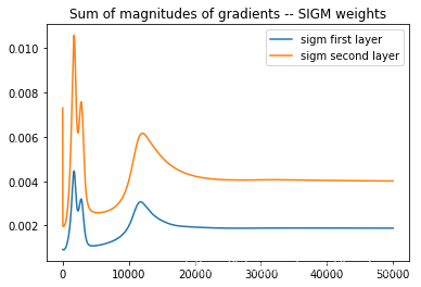
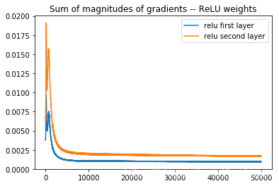
梯度消失问题

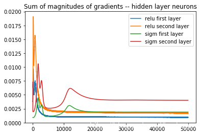
可以使用梯度大小的和作为隐藏层之间权重的一个简单的启发式来度量学习速度(也可以使用这里隐藏层中每个神经元的梯度大小)。直觉上，当权重向量或每个神经元的梯度值较大时，网络的学习速度较快。

plt.plot(np.array(sigm_array_1))
plt.plot(np.array(sigm_array_2))
plt.title('Sum of magnitudes of gradients -- SIGM weights')
plt.legend(("sigm first layer", "sigm second layer"))

OUTPUT:

plt.plot(np.array(relu_array_1))
plt.plot(np.array(relu_array_2))
plt.title('Sum of magnitudes of gradients -- ReLU weights')
plt.legend(("relu first layer", "relu second layer"))

OUTPUT:

# Overlaying the two plots to compare
plt.plot(np.array(relu_array_1))
plt.plot(np.array(relu_array_2))
plt.plot(np.array(sigm_array_1))
plt.plot(np.array(sigm_array_2))
plt.title('Sum of magnitudes of gradients -- hidden layer neurons')
plt.legend(("relu first layer", "relu second layer","sigm first layer", "sigm second layer"))

OUTPUT:

分类器

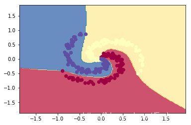
# plot the classifiers- SIGMOID
h = 0.02
x_min, x_max = X[:, 0].min() - 1, X[:, 0].max() + 1
y_min, y_max = X[:, 1].min() - 1, X[:, 1].max() + 1
xx, yy = np.meshgrid(np.arange(x_min, x_max, h),
                     np.arange(y_min, y_max, h))
Z = np.dot(sigmoid(np.dot(sigmoid(np.dot(np.c_[xx.ravel(), yy.ravel()], s_W1) + s_b1), s_W2) + s_b2), s_W3) + s_b3
Z = np.argmax(Z, axis=1)
Z = Z.reshape(xx.shape)
fig = plt.figure()
plt.contourf(xx, yy, Z, cmap=plt.cm.Spectral, alpha=0.8)
plt.scatter(X[:, 0], X[:, 1], c=y, s=40, cmap=plt.cm.Spectral)
plt.xlim(xx.min(), xx.max())
plt.ylim(yy.min(), yy.max())

OUTPUT:

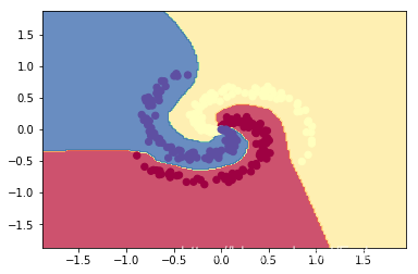
# plot the classifiers-- RELU
h = 0.02
x_min, x_max = X[:, 0].min() - 1, X[:, 0].max() + 1
y_min, y_max = X[:, 1].min() - 1, X[:, 1].max() + 1
xx, yy = np.meshgrid(np.arange(x_min, x_max, h),
                     np.arange(y_min, y_max, h))
Z = np.dot(relu(np.dot(relu(np.dot(np.c_[xx.ravel(), yy.ravel()], r_W1) + r_b1), r_W2) + r_b2), r_W3) + r_b3
Z = np.argmax(Z, axis=1)
Z = Z.reshape(xx.shape)
fig = plt.figure()
plt.contourf(xx, yy, Z, cmap=plt.cm.Spectral, alpha=0.8)
plt.scatter(X[:, 0], X[:, 1], c=y, s=40, cmap=plt.cm.Spectral)
plt.xlim(xx.min(), xx.max())
plt.ylim(yy.min(), yy.max())

OUTPUT: