基于树结构的机器学习模型

基于树结构的机器学习模型

在深度学习被广泛应用之前，基于树形结构的机器学习模型，比如说决策树，随机森林，GBDT，Xgboost等等被广泛的应用到分类等常见场景中，下面总结一下常见一个一些树形结构的机器学习模型。

1：决策树

常见的决策树算法有ID3，C4.5，CART(classification and regression tree)等等。由于存在很多好的文章已经详细的介绍了这些算法，如深入浅出理解决策树算法（二）-ID3算法与C4.5算法等等，这里主要写出我的一些理解。

ID3算法使用的信息增益：

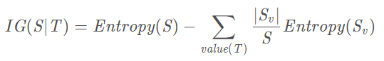
其实决策树中所言的information gain就是属性与类的互信息。由于ID3算法的信息增益计算出来后，那些具有更多可选取值的属性带来的信息增益往往更大，因此倾向于选择这些属性。但是存在一个问题，根据这些属性划分的节点往往包含的个数比较少，带来的效果不好。类比，这种现象有点像图割算法，MinCut最初的目标函数往往会将孤立的点划分出来，因此后面的NormalizedCut在目标函数中将子图的大小考虑进来，解决了这个问题。

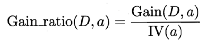
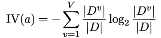
后来的C4.5算法使用信息增益率作为划分节点的标准，可以看出，正则化系数IV实际上是属性个数的熵，属性个数越多，熵越大，因此也是一个正则化。

class DecitionTree():
    """This is a decision tree classifier. """
    
    def __init__(self, criteria='ID3'):
        self._tree = None
        if criteria == 'ID3' or criteria == 'C4.5':
            self._criteria = criteria
        else:
            raise Exception("criterion should be ID3 or C4.5")
    
    def _calEntropy(slef, y):
        '''
        功能：_calEntropy用于计算香农熵 e=-sum(pi*log pi)
        参数：其中y为数组array
        输出：信息熵entropy
        '''
        n = y.shape[0]  
        labelCounts = {}
        for label in y:
            if label not in labelCounts.keys():
                labelCounts[label] = 1
            else:
                labelCounts[label] += 1
        entropy = 0.0
        for key in labelCounts:
            prob = float(labelCounts[key])/n
            entropy -= prob * np.log2(prob)
        return entropy
    
    def _splitData(self, X, y, axis, cutoff):
        """
        参数：X为特征,y为label,axis为某个特征的下标,cutoff是下标为axis特征取值值
        输出：返回数据集中特征下标为axis，特征值等于cutoff的子数据集
        """
        ret = []
        featVec = X[:,axis]
        n = X.shape[1]      #特征个数
        X = X[:,[i for i in range(n) if i!=axis]]
        for i in range(len(featVec)):
            if featVec[i] == cutoff:
                ret.append(i)
        return X[ret, :], y[ret]   
            
    def _chooseBestSplit(self, X, y):
        """ID3 & C4.5
        参数：X为特征，y为label
        功能：根据信息增益或者信息增益率来获取最好的划分特征
        输出：返回最好划分特征的下标
        """
        numFeat = X.shape[1]
        baseEntropy = self._calEntropy(y)
        bestSplit = 0.0
        best_idx  = -1
        for i in range(numFeat):
            featlist = X[:,i]   #得到第i个特征对应的特征列
            uniqueVals = set(featlist)
            curEntropy = 0.0
            splitInfo = 0.0
            for value in uniqueVals:
                sub_x, sub_y = self._splitData(X, y, i, value)
                prob = len(sub_y)/float(len(y))      #计算某个特征的某个值的概率
                curEntropy += prob * self._calEntropy(sub_y)    #迭代计算条件熵
                splitInfo -=  prob * np.log2(prob) #分裂信息，用于计算信息增益率
            IG = baseEntropy - curEntropy
            if self._criteria=="ID3":
                if IG > bestSplit:
                    bestSplit = IG
                    best_idx = i
            if self._criteria=="C4.5":
                if splitInfo == 0.0:
                    pass
                IGR = IG/splitInfo
                if IGR > bestSplit:
                    bestSplit = IGR
                    best_idx = i
        return best_idx
        
    def _majorityCnt(self, labellist):
        """
        参数:labellist是类标签，序列类型为list
        输出：返回labellist中出现次数最多的label
        """
        labelCount={}
        for vote in labellist:
            if vote not in labelCount.keys(): 
                labelCount[vote] = 0
            labelCount[vote] += 1
        sortedClassCount = sorted(labelCount.iteritems(), key=lambda x:x[1], \
                                     reverse=True)
        return sortedClassCount[0][0]

    def _createTree(self, X, y, featureIndex):
        """
        参数:X为特征,y为label,featureIndex类型是元组，记录X特征在原始数据中的下标
        输出:根据当前的featureIndex创建一颗完整的树
        """
        labelList = list(y)
        if labelList.count(labelList[0]) == len(labelList): 
            return labelList[0]
        if len(featureIndex) == 0:
            return self._majorityCnt(labelList)
        bestFeatIndex = self._chooseBestSplit(X,y)
        bestFeatAxis = featureIndex[bestFeatIndex]
        featureIndex = list(featureIndex)
        featureIndex.remove(bestFeatAxis)
        featureIndex = tuple(featureIndex)
        myTree = {bestFeatAxis:{}}
        featValues = X[:, bestFeatIndex]
        uniqueVals = set(featValues)
        for value in uniqueVals:
            #对每个value递归地创建树
            sub_X, sub_y = self._splitData(X,y, bestFeatIndex, value)
            myTree[bestFeatAxis][value] = self._createTree(sub_X, sub_y, \
                                            featureIndex)
        return myTree  
        
    def fit(self, X, y):
        """
        参数：X是特征，y是类标签
        注意事项：对数据X和y进行类型检测，保证其为array
        输出：self本身
        """
        if isinstance(X, np.ndarray) and isinstance(y, np.ndarray):
            pass
        else:
            try:
                X = np.array(X)
                y = np.array(y)
            except:
                raise TypeError("numpy.ndarray required for X,y")
        featureIndex  = tuple(['x'+str(i) for i in range(X.shape[1])])
        self._tree = self._createTree(X,y,featureIndex)
        return self  #allow using: clf.fit().predict()
        
    def _classify(self, tree, sample):
        """
        用训练好的模型对输入数据进行分类 
        注意：决策树的构建是一个递归的过程，用决策树分类也是一个递归的过程
        _classify()一次只能对一个样本（sample）分类
        """
        featIndex = tree.keys()[0] #得到数的根节点值
        secondDict = tree[featIndex] #得到以featIndex为划分特征的结果
        axis=featIndex[1:] #得到根节点特征在原始数据中的下标
        key = sample[int(axis)] #获取待分类样本中下标为axis的值
        valueOfKey = secondDict[key] #获取secondDict中keys为key的value值
        if type(valueOfKey).__name__=='dict': #如果value为dict，则继续递归分类
            return self._classify(valueOfKey, sample)
        else: 
            return valueOfKey
        
    def predict(self, X):
        if self._tree==None:
            raise NotImplementedError("Estimator not fitted, call `fit` first")
        #对X的类型进行检测，判断其是否是数组
        if isinstance(X, np.ndarray): 
            pass
        else: 
            try:
                X = np.array(X)
            except:
                raise TypeError("numpy.ndarray required for X")
            
        if len(X.shape) == 1:
            return self._classify(self._tree, X)
        else:
            result = []
            for i in range(X.shape[0]):
                value = self._classify(self._tree, X[i])
                print str(i+1)+"-th sample is classfied as:", value 
                result.append(value)
            return np.array(result)

    def show(self, outpdf):
        if self._tree==None:
            pass
        #plot the tree using matplotlib
        import treePlotter
        treePlotter.createPlot(self._tree, outpdf)
    
if __name__=="__main__":
    trainfile=r"data\train.txt"
    testfile=r"data\test.txt"
    import sys
    sys.path.append(r"F:\CSU\Github\MachineLearning\lib")  
    import dataload as dload
    train_x, train_y = dload.loadData(trainfile)
    test_x, test_y = dload.loadData(testfile)
    
    clf = DecitionTree(criteria="C4.5")
    clf.fit(train_x, train_y)
    result = clf.predict(test_x)    
    outpdf = r"tree.pdf"
    clf.show(outpdf)

 上面的代码来自于decisionTree，是比较简单的ID3,C4.5实现。可以知道，ID3、C4.5只用于分类任务，因为不管是信息增益还是信息增益率都是基于类别标签计算的。而CART树既可以做分类，也可以做回归，下面是CART分类树的简单的实现代码，来自于How To Implement The Decision Tree Algorithm From Scratch In Python - MachineLearningMastery.com。

# CART on the Bank Note dataset
from random import seed
from random import randrange
from csv import reader

# Load a CSV file
def load_csv(filename):
	file = open(filename, "rb")
	lines = reader(file)
	dataset = list(lines)
	return dataset

# Convert string column to float
def str_column_to_float(dataset, column):
	for row in dataset:
		row[column] = float(row[column].strip())

# Split a dataset into k folds
def cross_validation_split(dataset, n_folds):
	dataset_split = list()
	dataset_copy = list(dataset)
	fold_size = int(len(dataset) / n_folds)
	for i in range(n_folds):
		fold = list()
		while len(fold) < fold_size:
			index = randrange(len(dataset_copy))
			fold.append(dataset_copy.pop(index))
		dataset_split.append(fold)
	return dataset_split

# Calculate accuracy percentage
def accuracy_metric(actual, predicted):
	correct = 0
	for i in range(len(actual)):
		if actual[i] == predicted[i]:
			correct += 1
	return correct / float(len(actual)) * 100.0

# Evaluate an algorithm using a cross validation split
def evaluate_algorithm(dataset, algorithm, n_folds, *args):
	folds = cross_validation_split(dataset, n_folds)
	scores = list()
	for fold in folds:
		train_set = list(folds)
		train_set.remove(fold)
		train_set = sum(train_set, [])
		test_set = list()
		for row in fold:
			row_copy = list(row)
			test_set.append(row_copy)
			row_copy[-1] = None
		predicted = algorithm(train_set, test_set, *args)
		actual = [row[-1] for row in fold]
		accuracy = accuracy_metric(actual, predicted)
		scores.append(accuracy)
	return scores

# Split a dataset based on an attribute and an attribute value
def test_split(index, value, dataset):
	left, right = list(), list()
	for row in dataset:
		if row[index] < value:
			left.append(row)
		else:
			right.append(row)
	return left, right

# Calculate the Gini index for a split dataset
def gini_index(groups, classes):
	# count all samples at split point
	n_instances = float(sum([len(group) for group in groups]))
	# sum weighted Gini index for each group
	gini = 0.0
	for group in groups:
		size = float(len(group))
		# avoid divide by zero
		if size == 0:
			continue
		score = 0.0
		# score the group based on the score for each class
		for class_val in classes:
			p = [row[-1] for row in group].count(class_val) / size
			score += p * p
		# weight the group score by its relative size
		gini += (1.0 - score) * (size / n_instances)
	return gini

# Select the best split point for a dataset
def get_split(dataset):
	class_values = list(set(row[-1] for row in dataset))
	b_index, b_value, b_score, b_groups = 999, 999, 999, None
	for index in range(len(dataset[0])-1):
		for row in dataset:
			groups = test_split(index, row[index], dataset)
			gini = gini_index(groups, class_values)
			if gini < b_score:
				b_index, b_value, b_score, b_groups = index, row[index], gini, groups
	return {'index':b_index, 'value':b_value, 'groups':b_groups}

# Create a terminal node value
def to_terminal(group):
	outcomes = [row[-1] for row in group]
	return max(set(outcomes), key=outcomes.count)

# Create child splits for a node or make terminal
def split(node, max_depth, min_size, depth):
	left, right = node['groups']
	del(node['groups'])
	# check for a no split
	if not left or not right:
		node['left'] = node['right'] = to_terminal(left + right)
		return
	# check for max depth
	if depth >= max_depth:
		node['left'], node['right'] = to_terminal(left), to_terminal(right)
		return
	# process left child
	if len(left) <= min_size:
		node['left'] = to_terminal(left)
	else:
		node['left'] = get_split(left)
		split(node['left'], max_depth, min_size, depth+1)
	# process right child
	if len(right) <= min_size:
		node['right'] = to_terminal(right)
	else:
		node['right'] = get_split(right)
		split(node['right'], max_depth, min_size, depth+1)

# Build a decision tree
def build_tree(train, max_depth, min_size):
	root = get_split(train)
	split(root, max_depth, min_size, 1)
	return root

# Make a prediction with a decision tree
def predict(node, row):
	if row[node['index']] < node['value']:
		if isinstance(node['left'], dict):
			return predict(node['left'], row)
		else:
			return node['left']
	else:
		if isinstance(node['right'], dict):
			return predict(node['right'], row)
		else:
			return node['right']

# Classification and Regression Tree Algorithm
def decision_tree(train, test, max_depth, min_size):
	tree = build_tree(train, max_depth, min_size)
	predictions = list()
	for row in test:
		prediction = predict(tree, row)
		predictions.append(prediction)
	return(predictions)

# Test CART on Bank Note dataset
seed(1)
# load and prepare data
filename = 'data_banknote_authentication.csv'
dataset = load_csv(filename)
# convert string attributes to integers
for i in range(len(dataset[0])):
	str_column_to_float(dataset, i)
# evaluate algorithm
n_folds = 5
max_depth = 5
min_size = 10
scores = evaluate_algorithm(dataset, decision_tree, n_folds, max_depth, min_size)
print('Scores: %s' % scores)
print('Mean Accuracy: %.3f%%' % (sum(scores)/float(len(scores))))

上面的CART数是分类树，使用的Gini系数作为属性选择的指标，要是是回归树的话，使用mse作为指标就行了。 ML-From-Scratch上有一个更好的决策树以及回归树的实现方法。

2：GBDT

梯度提升（Gradient boost）树的基本概念就是建立多棵树，分别将一个待分类的数据x输入到这些树中，将得到的结果进行累加求和（加法模型），和随机森林（bagging）使用投票的方法不同。

 那么怎么选择f呢？梯度提升树使用损失函数的负梯度的值作为当前叶子结点的值（如果非叶子节点，那么会继续分割，因此不存在值），注意梯度是关于上一次（当前）的预测值得到的，GBDT一般用于回归的时候使用的是MSE作为损失函数（损失函数实际上就是在选择分割属性的时候，使用损失函数衡量所选属性及其具体值的好坏），分类的时候使用交叉熵损失函数，除此之外，分类的时候会把离散的标签(如category)转换成onehot当做回归来做。下面是GBDT的代码，来自于https://github.com/eriklindernoren/ML-From-Scratch。

class GradientBoosting(object):
    """Super class of GradientBoostingClassifier and GradientBoostinRegressor. 
    Uses a collection of regression trees that trains on predicting the gradient
    of the loss function. 
    Parameters:
    -----------
    n_estimators: int
        The number of classification trees that are used.
    learning_rate: float
        The step length that will be taken when following the negative gradient during
        training.
    min_samples_split: int
        The minimum number of samples needed to make a split when building a tree.
    min_impurity: float
        The minimum impurity required to split the tree further. 
    max_depth: int
        The maximum depth of a tree.
    regression: boolean
        True or false depending on if we're doing regression or classification.
    """
    def __init__(self, n_estimators, learning_rate, min_samples_split,
                 min_impurity, max_depth, regression):
        self.n_estimators = n_estimators
        self.learning_rate = learning_rate
        self.min_samples_split = min_samples_split
        self.min_impurity = min_impurity
        self.max_depth = max_depth
        self.regression = regression
        self.bar = progressbar.ProgressBar(widgets=bar_widgets)
        
        # Square loss for regression
        # Log loss for classification
        self.loss = SquareLoss()
        if not self.regression:
            self.loss = CrossEntropy()

        # Initialize regression trees
        self.trees = []
        for _ in range(n_estimators):
            tree = RegressionTree(
                    min_samples_split=self.min_samples_split,
                    min_impurity=min_impurity,
                    max_depth=self.max_depth)
            self.trees.append(tree)


    def fit(self, X, y):
        y_pred = np.full(np.shape(y), np.mean(y, axis=0))
        for i in self.bar(range(self.n_estimators)):
            gradient = self.loss.gradient(y, y_pred)
            self.trees[i].fit(X, gradient)
            update = self.trees[i].predict(X)
            # Update y prediction
            y_pred -= np.multiply(self.learning_rate, update)


    def predict(self, X):
        y_pred = np.array([])
        # Make predictions
        for tree in self.trees:
            update = tree.predict(X)
            update = np.multiply(self.learning_rate, update)
            y_pred = -update if not y_pred.any() else y_pred - update

        if not self.regression:
            # Turn into probability distribution
            y_pred = np.exp(y_pred) / np.expand_dims(np.sum(np.exp(y_pred), axis=1), axis=1)
            # Set label to the value that maximizes probability
            y_pred = np.argmax(y_pred, axis=1)
        return y_pred


class GradientBoostingRegressor(GradientBoosting):
    def __init__(self, n_estimators=200, learning_rate=0.5, min_samples_split=2,
                 min_var_red=1e-7, max_depth=4, debug=False):
        super(GradientBoostingRegressor, self).__init__(n_estimators=n_estimators, 
            learning_rate=learning_rate, 
            min_samples_split=min_samples_split, 
            min_impurity=min_var_red,
            max_depth=max_depth,
            regression=True)

class GradientBoostingClassifier(GradientBoosting):
    def __init__(self, n_estimators=200, learning_rate=.5, min_samples_split=2,
                 min_info_gain=1e-7, max_depth=2, debug=False):
        super(GradientBoostingClassifier, self).__init__(n_estimators=n_estimators, 
            learning_rate=learning_rate, 
            min_samples_split=min_samples_split, 
            min_impurity=min_info_gain,
            max_depth=max_depth,
            regression=False)

    def fit(self, X, y):
        y = to_categorical(y)
        super(GradientBoostingClassifier, self).fit(X, y)

3：xgboost

xgboost实际上也是梯度提升树，只不过作者在实现的时候加入了很多特性，比如说分布式求解之类的，这些特性我暂时了解的不深，在这里主要是对xgboost的基本算法进行一些说明。

定义函数的二阶泰勒展开：

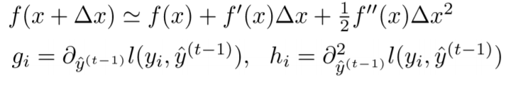
梯度提升树的损失函数可以写作：

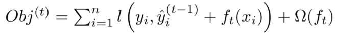
其中第一项是偏差，第二项是正则项。我们将第一项损失函数进行泰勒展开可以得到：

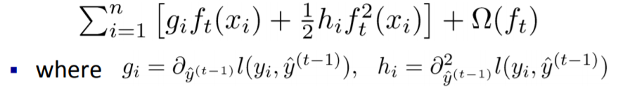
 因为是常数，所以可以进一步简化为：

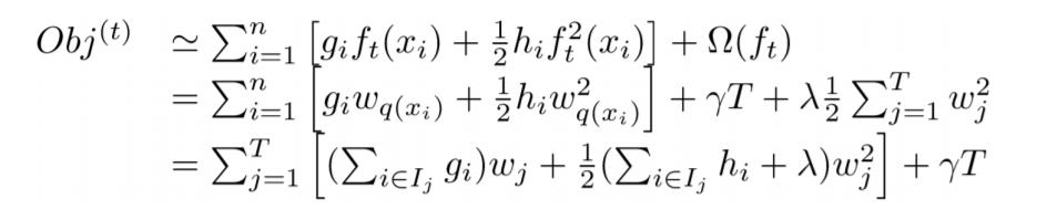
把上式再次进行一些变换可以得到：

 上式存在闭合解：

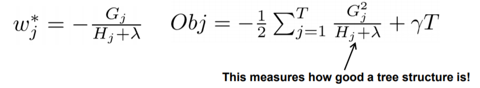
 其中左边一项用于替代GBDT中的负梯度作为叶子结点的值，右边一项作为目标函数用于衡量节点划分的好坏。

class LogisticLoss():
    def __init__(self):
        sigmoid = Sigmoid()
        self.log_func = sigmoid
        self.log_grad = sigmoid.gradient

    def loss(self, y, y_pred):
        y_pred = np.clip(y_pred, 1e-15, 1 - 1e-15)
        p = self.log_func(y_pred)
        return y * np.log(p) + (1 - y) * np.log(1 - p)

    # gradient w.r.t y_pred
    def gradient(self, y, y_pred):
        p = self.log_func(y_pred)
        return -(y - p)

    # w.r.t y_pred
    def hess(self, y, y_pred):
        p = self.log_func(y_pred)
        return p * (1 - p)


class XGBoost(object):
    """The XGBoost classifier.
    Reference: http://xgboost.readthedocs.io/en/latest/model.html
    Parameters:
    -----------
    n_estimators: int
        The number of classification trees that are used.
    learning_rate: float
        The step length that will be taken when following the negative gradient during
        training.
    min_samples_split: int
        The minimum number of samples needed to make a split when building a tree.
    min_impurity: float
        The minimum impurity required to split the tree further. 
    max_depth: int
        The maximum depth of a tree.
    """
    def __init__(self, n_estimators=200, learning_rate=0.001, min_samples_split=2,
                 min_impurity=1e-7, max_depth=2):
        self.n_estimators = n_estimators            # Number of trees
        self.learning_rate = learning_rate          # Step size for weight update
        self.min_samples_split = min_samples_split  # The minimum n of sampels to justify split
        self.min_impurity = min_impurity              # Minimum variance reduction to continue
        self.max_depth = max_depth                  # Maximum depth for tree

        self.bar = progressbar.ProgressBar(widgets=bar_widgets)
        
        # Log loss for classification
        self.loss = LogisticLoss()

        # Initialize regression trees
        self.trees = []
        for _ in range(n_estimators):
            tree = XGBoostRegressionTree(
                    min_samples_split=self.min_samples_split,
                    min_impurity=min_impurity,
                    max_depth=self.max_depth,
                    loss=self.loss)

            self.trees.append(tree)

    def fit(self, X, y):
        y = to_categorical(y)

        y_pred = np.zeros(np.shape(y))
        for i in self.bar(range(self.n_estimators)):
            tree = self.trees[i]
            y_and_pred = np.concatenate((y, y_pred), axis=1)
            tree.fit(X, y_and_pred)
            update_pred = tree.predict(X)

            y_pred -= np.multiply(self.learning_rate, update_pred)

    def predict(self, X):
        y_pred = None
        # Make predictions
        for tree in self.trees:
            # Estimate gradient and update prediction
            update_pred = tree.predict(X)
            if y_pred is None:
                y_pred = np.zeros_like(update_pred)
            y_pred -= np.multiply(self.learning_rate, update_pred)

        # Turn into probability distribution (Softmax)
        y_pred = np.exp(y_pred) / np.sum(np.exp(y_pred), axis=1, keepdims=True)
        # Set label to the value that maximizes probability
        y_pred = np.argmax(y_pred, axis=1)
        return y_pred

备注：

和神经网络相比，基于树模型的算法的优点在于，不需要进行一些额外的特征预处理，比如说scaling（正则化，归一化）等，不同维度特征之间的scale不会对结果进行影响，除此之外，树模型更加好解释，神经网络的解释性差。

参考文献：

怎么选择决策树还是神经网络

/BoostedTree