机器学习算法

机器学习算法

1：线性回归的解释

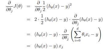
线性回归是最简单的机器学习算法之一，但是非常常用。我们都知道给定(x,y)作为训练数据，使用如下的目标函数进行优化：

然后使用优化方法，比如说梯度下降算法（或者牛顿法等）对上面的目标进行优化：

但是为什么直接使用平方差作为损失函数能够进行先行回归？下面的解释来自与Andrew Ng的机器学习课程：

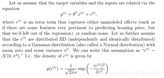
假设回归结果与真实值之间的误差满足正太分布（为什么满足正态分布，因为根据中心极限定理可知，任意多的随机变量的和满足正太分布），因此，可以得到下面的公式：

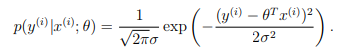
然后使用最大似然函数可以得到下面的结果：

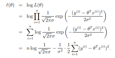
和KL散度与交叉熵的关系一样，从上面的式子可以得到，最大化似然函数等价于最小化平方差。但是为什么使用最大似然能够作为目标函数呢？从最上面的误差满足正态分布来说，我们希望误差尽可能的小，误差越小的话，对应的概率越大，因此最大化似然带来的结果就是误差最下。 

很多人认为伯努利分布或者sofamax分布的负对数似然表示交叉熵，但是实际上，任意一个负对数似然组成的损失都是在训练集上经验分布和定义在模型上概率分布之间的交叉熵，比如说上面的均方误差实际上就是经验分布和高斯分布之间的交叉熵。最大似然估计被证明，当样本数目m区域无穷大的时候，最大似然估计就收敛率而言是最好的渐进估计（偏差趋于0），因此实际上好多损失函数都是通过最大似然推导而来的。

2：超参数优化方法

1）交叉验证

交叉验证可以帮助我们手动的选择超参数。https://scikit-learn.org/stable/modules/cross_validation.html#cross-validation介绍了交叉验证的一些算法，以及在scikit-learn中的实现。

2）网格搜索(grid search)

网格搜索就是将所有的超参数的组合进行验证，使用交叉验证的方法，看验证集上面的效果怎么样，然后选择效果最好的超参数组合最为最终的结果。https://scikit-learn.org/stable/modules/grid_search.html介绍了scikit-learn里面实现的网格搜索算法。

https://scikit-learn.org/stable/auto_examples/model_selection/plot_randomized_search.html#sphx-glr-auto-examples-model-selection-plot-randomized-search-py对比了传统网格搜索和随机搜索的性能差异。

3）贝叶斯优化

https://arxiv.org/pdf/1012.2599.pdf

http://krasserm.github.io/2018/03/21/bayesian-optimization/

3：推荐系统

推荐算法在各种平台上面都能看见，头条的推荐，腾讯的用户推荐等等，Netflix在推荐系统的构建上面比较领先，下面介绍几种常用的推荐系统算法：

1）矩阵分解(matrix factorization)

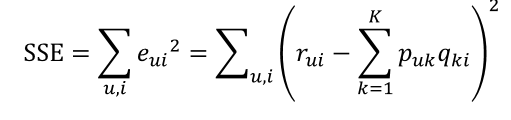
下面的矩阵是一个常见的用户-商品打分矩阵，?代表值的缺失。

 

 

下面的使用梯度下降进行矩阵分解的方法最早被simon在Netflix的推荐大赛上提出，后来被广泛使用。该方法和SVD没有什么联系，但是有时候基于矩阵分解的推荐算法会被称做为SVD，原因在这里。原话如下：

Let’s start by pointing out that the method usually referred to as “SVD” that is used in the context of recommendations is not strictly speaking the mathematical Singular Value Decomposition of a matrix but rather an approximate way to compute the low-rank approximation of the matrix by minimizing the squared error loss. A more accurate, albeit more generic, way to call this would be Matrix Factorization. The initial version of this approach in the context of the Netflix Prize was presented by Simon Funk in his famous Try This at Home blogpost. It is important to note that the “true SVD” approach had been indeed applied to the same task years before, with not so much practical success.

我在github记录了一版简单的基于矩阵分解的算法，和论文"MATRIX FACTORIZATION TECHNIQUES FOR RECOMMENDER
SYSTEMS"里面记录的初步版本一致。

def sgd(data_matrix, user, item, alpha, lam, iter_num):

    for j in range(iter_num):
        for u in range(data_matrix.shape[0]):
            for i in range(data_matrix.shape[1]):
                if data_matrix[u][i] != 0:
                    e_ui = data_matrix[u][i] - sum(user[u,:] * item[i,:])
                    user[u,:] += alpha * (e_ui * item[i,:] - lam * user[u,:])
                    item[i,:] += alpha * (e_ui * user[u,:] - lam * item[i,:])
    return user, item

import numpy
import sys


def run_demo(args):
    print args
    data = args[1]
    model = ProductRecommender()
    model.fit(data)


class ProductRecommender(object):
    """
    Generates recommendations using the matrix factorization approach.
    Derived and implemented from the Netflix paper.
    Author: William Falcon
    Has 2 modes:
    Mode A: Derives P, Q matrices intrinsically for k features.
    Use this approach to learn the features.
    Mode B: Derives P matrix given a constant P matrix (Products x features). Use this if you want to
    try the approach of selecting the features yourself.
    Example 1:
    from matrix_factor_model import ProductRecommender
    modelA = ProductRecommender()
    data = [[1,2,3], [0,2,3]]
    modelA.fit(data)
    model.predict_instance(1)
    # prints array([ 0.9053102 ,  2.02257811,  2.97001565])
    Model B example
    modelB = ProductRecommender()
    data = [[1,2,3], [0,2,3]]
    # product x features
    Q = [[2,3], [2, 4], [5, 9]]
    # fit
    modelA.fit(data, Q)
    model.predict_instance(1)
    # prints array([ 0.9053102 ,  2.02257811,  2.97001565])
    """

    def __init__(self):
        self.Q = None
        self.P = None

    def fit(self, user_x_product, latent_features_guess=2, learning_rate=0.0002, steps=5000, regularization_penalty=0.02, convergeance_threshold=0.001):
        """
        Trains the predictor with the given parameters.
        :param user_x_product:
        :param latent_features_guess:
        :param learning_rate:
        :param steps:
        :param regularization_penalty:
        :param convergeance_threshold:
        :return:
        """
        print 'training model...'
        return self.__factor_matrix(user_x_product, latent_features_guess, learning_rate, steps, regularization_penalty, convergeance_threshold)

    def predict_instance(self, row_index):
        """
        Returns all predictions for a given row
        :param row_index:
        :return:
        """
        return numpy.dot(self.P[row_index, :], self.Q.T)

    def predict_all(self):
        """
        Returns the full prediction matrix
        :return:
        """
        return numpy.dot(self.P, self.Q.T)

    def get_models(self):
        """
        Returns a copy of the models
        :return:
        """
        return self.P, self.Q

    def __factor_matrix(self, R, K, alpha, steps, beta, error_limit):
        """
        R = user x product matrix
        K = latent features count (how many features we think the model should derive)
        alpha = learning rate
        beta = regularization penalty (minimize over/under fitting)
        step = logistic regression steps
        error_limit = algo finishes when error reaches this level
        Returns:
        P = User x features matrix. (How strongly a user is associated with a feature)
        Q = Product x feature matrix. (How strongly a product is associated with a feature)
        To predict, use dot product of P, Q
        """
        # Transform regular array to numpy array
        R = numpy.array(R)

        # Generate P - N x K
        # Use random values to start. Best performance
        N = len(R)
        M = len(R[0])
        P = numpy.random.rand(N, K)

        # Generate Q - M x K
        # Use random values to start. Best performance
        Q = numpy.random.rand(M, K)
        Q = Q.T

        error = 0

        # iterate through max # of steps
        for step in xrange(steps):

            # iterate each cell in r
            for i in xrange(len(R)):
                for j in xrange(len(R[i])):
                    if R[i][j] > 0:

                        # get the eij (error) side of the equation
                        eij = R[i][j] - numpy.dot(P[i, :], Q[:, j])

                        for k in xrange(K):
                            # (*update_rule) update pik_hat
                            P[i][k] = P[i][k] + alpha * (2 * eij * Q[k][j] - beta * P[i][k])

                            # (*update_rule) update qkj_hat
                            Q[k][j] = Q[k][j] + alpha * ( 2 * eij * P[i][k] - beta * Q[k][j] )

            # Measure error
            error = self.__error(R, P, Q, K, beta)

            # Terminate when we converge
            if error < error_limit:
                break

        # track Q, P (learned params)
        # Q = Products x feature strength
        # P = Users x feature strength
        self.Q = Q.T
        self.P = P

        self.__print_fit_stats(error, N, M)

    def __error(self, R, P, Q, K, beta):
        """
        Calculates the error for the function
        :param R:
        :param P:
        :param Q:
        :param K:
        :param beta:
        :return:
        """
        e = 0
        for i in xrange(len(R)):
            for j in xrange(len(R[i])):
                if R[i][j] > 0:

                    # loss function error sum( (y-y_hat)^2 )
                    e = e + pow(R[i][j]-numpy.dot(P[i,:],Q[:,j]), 2)

                    # add regularization
                    for k in xrange(K):

                        # error + ||P||^2 + ||Q||^2
                        e = e + (beta/2) * ( pow(P[i][k], 2) + pow(Q[k][j], 2) )
        return e

    def __print_fit_stats(self, error, samples_count, products_count):
        print 'training complete...'
        print '------------------------------'
        print 'Stats:'
        print 'Error: %0.2f' % error
        print 'Samples: ' + str(samples_count)
        print 'Products: ' + str(products_count)
        print '------------------------------'

if __name__ == '__main__':
    run_demo(sys.argv)

上面是最简单的目标函数，比较具体的介绍可以查看 参考文献第一篇。那么上面的基于矩阵分解的算法是没有用到SVD的，那么SVD什么时候被用到算法里面了呢？答案是，SVD在上面的推荐算法里面不会直接使用SVD分解，而是直接使用矩阵分解的思想，通过梯度下降算法优化目标函数（一般只使用存在打分的项，然后加入一些正则化项防止过拟合），surprise提供了SVD在推荐系统的一个实现，P,Q矩阵都是使用正太分布初始化，然后使用梯度下降进行优化的，详情可以查看https://surprise.readthedocs.io/en/stable/matrix_factorization.html#surprise.prediction_algorithms.matrix_factorization.SVD

因为一般打分矩阵是稀疏的，因此不能直接使用SVD分解，需要进行一些预处理，比如说缺失值填充等等，使用SVD分解同样可以得到上面的P,Q矩阵，然后被用到协同过滤算法里面，当做每个商品和用户的特征。

参考：

https://blog.youkuaiyun.com/zhongkejingwang/article/details/43083603

https://www.cnblogs.com/bjwu/p/9358777.html（*）

https://surprise.readthedocs.io/en/stable/matrix_factorization.html#surprise.prediction_algorithms.matrix_factorization.SVD

https://datajobs.com/data-science-repo/Recommender-Systems-[Netflix].pdf

2）RBM

SVD和RBM（受限制玻尔兹曼机）都是Netflix采用过的推荐算法。RBM是一个基于能量的算法，目的是使得从隐藏层重构回来的可见层数据能够和可见层数据的差异尽可能的小，实际上就是autoencoder的思想。但是RBM使用的是MLE（最大似然估计）作为目标，使用梯度下降来对参数进行优化的。

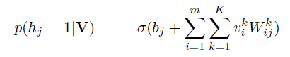
RBM之所以区别于BM的原因是隐藏层和课件层内部不存在连接，详情可查看https://www.cnblogs.com/pinard/p/6530523.html ，将RBM应用于推荐，可见层就是一个用户对所有商品的打分，需要进行如下的变种：

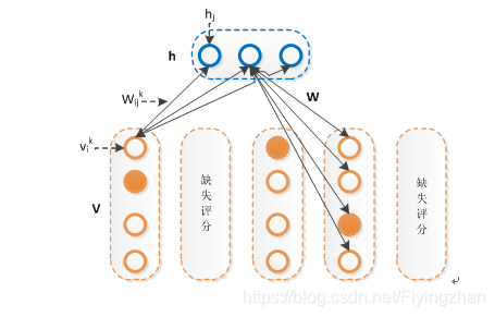
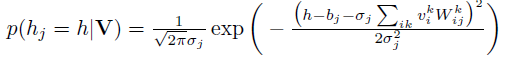
改进主要集中于可见层的输入，每个节点从二维的变为了一个k维的输入，如果对某些商品没有打分的话，节点的输入就都为0，相当于没有连接 ，使用最大似然作为目标函数进行优化。当训练好一个模型之后，我们输入一个用户的打分情况，会返回一个k维的实数向量，选择最大值，或者sofamax之后选择概率最大的一项，作为该商品的打分。对隐藏单元的先验概率的不同预测，存在伯努利RBM（下图2）和高斯RBM（下图1）：

下面是RBM的python实现代码（转自https://zhuanlan.zhihu.com/p/23970608）：

# coding:utf-8
import time
import numpy as np
import pandas as pd


class BRBM(object):
    def __init__(self, n_visible, n_hiddens=2, learning_rate=0.1, batch_size=10, n_iter=300):
        self.n_hiddens = n_hiddens
        self.learning_rate = learning_rate
        self.batch_size = batch_size
        self.n_iter = n_iter

        self.components_ = np.asarray(np.random.normal(0, 0.01, (n_hiddens, n_visible)), order='fortran')
        self.intercept_hidden_ = np.zeros(n_hiddens, )
        self.intercept_visible_ = np.zeros(n_visible, )
        self.h_samples_ = np.zeros((batch_size, n_hiddens))

    def transform(self, x):
        h = self._mean_hiddens(x)
        return h

    def reconstruct(self, x):
        h = self._mean_hiddens(x)
        v = self._mean_visible(h)
        return v

    def gibbs(self, v):
        h_ = self._sample_hiddens(v)
        v_ = self._sample_visibles(h_)
        return v_

    def fit(self, x):
        n_samples = x.shape[0]
        n_batches = int(np.ceil(float(n_samples) / self.batch_size))
        batch_slices = list(self._slices(n_batches * self.batch_size, n_batches, n_samples))
        for iteration in xrange(self.n_iter):
            for batch_slice in batch_slices:
                self._fit(x[batch_slice])
        return self

    def _sigmoid(self, x):
        return 1.0 / (1.0 + np.exp(-x))

    def _mean_hiddens(self, v):
        p = np.dot(v, self.components_.T)
        p += self.intercept_hidden_
        return self._sigmoid(p)

    def _mean_visible(self, h):
        p = np.dot(h, self.components_)
        p += self.intercept_visible_
        return self._sigmoid(p)

    def _sample_hiddens(self, v):
        p = self._mean_hiddens(v)
        return np.random.random_sample(size=p.shape) < p

    def _sample_visibles(self, h):
        p = self._mean_visible(h)
        return np.random.random_sample(size=p.shape) < p

    def _free_energy(self, v):
        return (- np.dot(v, self.intercept_visible_)
                - np.logaddexp(0, np.dot(v, self.components_.T)
                               + self.intercept_hidden_).sum(axis=1))

    def _fit(self, v_pos):
        h_pos = self._mean_hiddens(v_pos)
        v_neg = self._sample_visibles(self.h_samples_)  
        h_neg = self._mean_hiddens(v_neg)

        lr = float(self.learning_rate) / v_pos.shape[0]
        update = np.dot(v_pos.T, h_pos).T
        update -= np.dot(h_neg.T, v_neg)

        self.components_ += lr * update
        self.intercept_hidden_ += lr * (h_pos.sum(axis=0) - h_neg.sum(axis=0))
        self.intercept_visible_ += lr * (np.asarray(v_pos.sum(axis=0)).squeeze() - v_neg.sum(axis=0))
        h_neg[np.random.uniform(size=h_neg.shape) < h_neg] = 1.0  # sample binomial
        self.h_samples_ = np.floor(h_neg, h_neg)

    def _slices(self, n, n_packs, n_samples=None):
        start = 0  
        for pack_num in range(n_packs):
            this_n = n // n_packs
            if pack_num < n % n_packs:
                this_n += 1
            if this_n > 0:
                end = start + this_n
                if n_samples is not None:
                    end = min(n_samples, end)
                yield slice(start, end, None)
                start = end

参考：

https://github.com/meownoid/tensorfow-rbm（tensorflow构建rbm作为一个特征学习模型）

https://blog.youkuaiyun.com/u013414741/article/details/47151059

https://www.cnblogs.com/pinard/p/6530523.html

https://zhuanlan.zhihu.com/p/40120848

3）协同过滤算法

协同过滤算法是最早的推荐算法之一，分为基于用户和基于商品的协同过滤，主要是根据用户或者商品的相似度，对未知的商品得到一个打分的算法，可以查看https://blog.youkuaiyun.com/yimingsilence/article/details/54934302。

4：svd分解

奇异值分解是一个有着很明显的物理意义的一种方法，它可以将一个比较复杂的矩阵用更小更简单的几个子矩阵的相乘来表示，这些小矩阵描述的是矩阵的重要的特性。对于奇异值,它跟我们特征分解中的特征值类似，在奇异值矩阵中也是按照从大到小排列，而且奇异值的减少特别的快，在很多情况下，前10%甚至1%的奇异值的和就占了全部的奇异值之和的99%以上的比例。也就是说，我们也可以用最大的k个的奇异值和对应的左右奇异向量来近似描述矩阵。

特征值分解可以得到特征值与特征向量，特征值表示的是这个特征到底有多重要，而特征向量表示这个特征是什么，可以将每一组特征向量理解为一个线性的子空间，我们可以利用这些线性的子空间干很多的事情。 当矩阵是高维的情况下，那么这个矩阵就是高维空间下的一个线性变换，这个变换也同样有很多的变换方向，我们通过特征值分解得到的前N个特征向量，那么就对应了这个矩阵最主要的N个变化方向。我们利用这前N个变化方向，就可以近似这个矩阵（变换）。也就是之前说的：提取这个矩阵最重要的特征。

PCA的实现一般有两种，一种是用特征值分解去实现的，一种是用奇异值分解去实现的。SVD一般用于降维，生成一个矩阵减少计算量（比如说在PCA中使用SVD的一些trick可以避免求协方差矩阵）。

参考：

https://www.cnblogs.com/LeftNotEasy/archive/2011/01/19/svd-and-applications.html

https://www.cnblogs.com/pinard/p/6251584.html

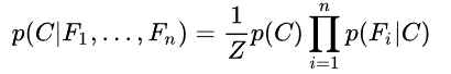
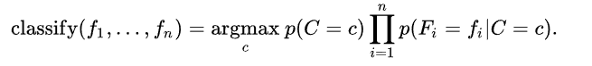
5：朴素贝叶斯

朴素贝叶斯中朴素的意思指的是输入数据X的每一维，我们认为其是不相关的。朴素贝叶斯算法主要分为以下几个步骤：

1：假设数据的概率分布是高斯（也可以假设为其他分布），根据类别将输入X分为c部分（c为类别的个数）；

2：根据每个部分求得该部分的均值和方差，作为该高斯分布的均值和方差；

3：将带预测数据x输入每个部分，根据贝叶斯公式（如下），得到似然值。似然值最大的类就是预测类。

 

class NaiveBayes():
    """The Gaussian Naive Bayes classifier. """
    def fit(self, X, y):
        self.X, self.y = X, y
        self.classes = np.unique(y)
        self.parameters = []
        # Calculate the mean and variance of each feature for each class
        for i, c in enumerate(self.classes):
            # Only select the rows where the label equals the given class
            X_where_c = X[np.where(y == c)]
            self.parameters.append([])
            # Add the mean and variance for each feature (column)
            for col in X_where_c.T:
                parameters = {"mean": col.mean(), "var": col.var()}
                self.parameters[i].append(parameters)

    def _calculate_likelihood(self, mean, var, x):
        """ Gaussian likelihood of the data x given mean and var """
        eps = 1e-4 # Added in denominator to prevent division by zero
        coeff = 1.0 / math.sqrt(2.0 * math.pi * var + eps)
        exponent = math.exp(-(math.pow(x - mean, 2) / (2 * var + eps)))
        return coeff * exponent

    def _calculate_prior(self, c):
        """ Calculate the prior of class c
        (samples where class == c / total number of samples)"""
        frequency = np.mean(self.y == c)
        return frequency

    def _classify(self, sample):
        """ Classification using Bayes Rule P(Y|X) = P(X|Y)*P(Y)/P(X),
            or Posterior = Likelihood * Prior / Scaling Factor
        P(Y|X) - The posterior is the probability that sample x is of class y given the
                 feature values of x being distributed according to distribution of y and the prior.
        P(X|Y) - Likelihood of data X given class distribution Y.
                 Gaussian distribution (given by _calculate_likelihood)
        P(Y)   - Prior (given by _calculate_prior)
        P(X)   - Scales the posterior to make it a proper probability distribution.
                 This term is ignored in this implementation since it doesn't affect
                 which class distribution the sample is most likely to belong to.
        Classifies the sample as the class that results in the largest P(Y|X) (posterior)
        """
        posteriors = []
        # Go through list of classes
        for i, c in enumerate(self.classes):
            # Initialize posterior as prior
            posterior = self._calculate_prior(c)
            # Naive assumption (independence):
            # P(x1,x2,x3|Y) = P(x1|Y)*P(x2|Y)*P(x3|Y)
            # Posterior is product of prior and likelihoods (ignoring scaling factor)
            for feature_value, params in zip(sample, self.parameters[i]):
                # Likelihood of feature value given distribution of feature values given y
                likelihood = self._calculate_likelihood(params["mean"], params["var"], feature_value)
                posterior *= likelihood
            posteriors.append(posterior)
        # Return the class with the largest posterior probability
        return self.classes[np.argmax(posteriors)]

    def predict(self, X):
        """ Predict the class labels of the samples in X """
        y_pred = [self._classify(sample) for sample in X]
        return y_pred