强化学习实战——Q learning 实现倒立摆

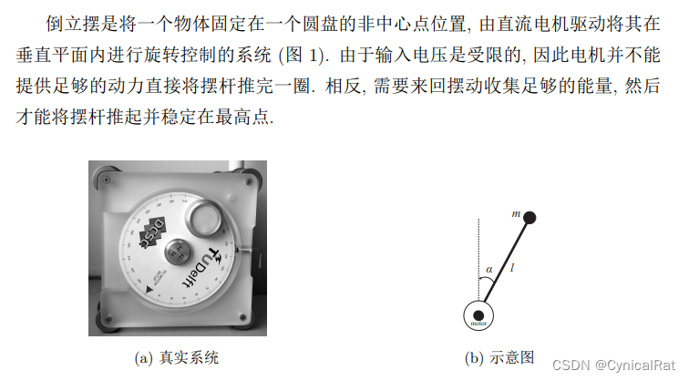
倒立摆参数以及数学模型

 

首先是写一个倒立摆的AGENT模型

pendulum_env.py

import numpy as np
import matplotlib.pyplot as plt
# import matplotlib
import matplotlib.animation as animation
# import IPython


class Pendulum:
    """
    构建一个倒立摆环境
    """

    def __init__(self):
        """
        初始化
        """
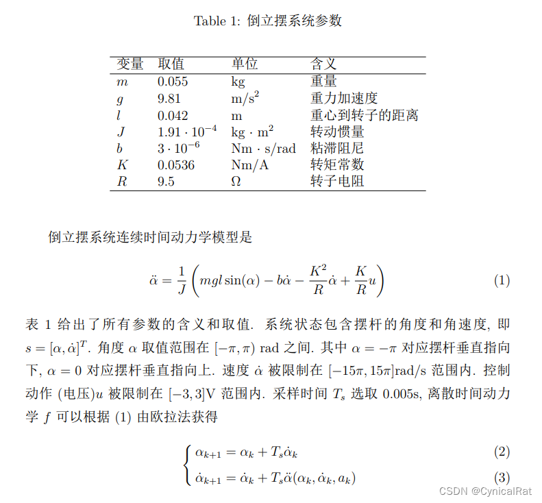
        # 倒立摆系统参数
        self._m = 0.055  # 转子重量
        self._g = 9.81  # 重力加速度
        self._l = 0.042  # 重心到转子距离
        self._J = 1.91e-4  # 转动惯量
        self._b = 3e-6  # 粘滞阻尼
        self._K = 0.0536  # 转矩常数
        self._R = 9.5  # 转子电阻

        # 状态维度 2维 角度angle和角速度angular
        self.state_dims = 2
        # 采样时间
        self.Ts = 0.005

        # 取值范围
        self.max_anger = np.pi  # 最大角度
        self.max_angular = 15 * np.pi  # 最大角速度
        self.max_voltage = 3  # 最大电压

    def get_delta_angular(self, x, u):
        """
        获取倒立摆角加速度
        :param x: 该时刻输入状态 [角度，角速度]
        :param u: 该时刻输入电压
        :return: 该时刻角加速度
        """
        temp = self._m * self._g * self._l * np.sin(x[0])
        _temp = (temp - self._b * x[1] - (self._K ** 2) * x[1] / self._R + self._K * u / self._R)
        return _temp / self._J

    def get_next_state(self, x, u):
        """
        根据离散时间动力学模型获得下次状态
        :param x: 该时刻输入状态 [角度，角速度]
        :param u: 该时刻输入电压
        :return: 下一时刻的新状态 [角度，角速度]
        """
        alpha = x[0] + self.Ts * x[1]
        d_alpha = x[1] + self.Ts * self.get_delta_angular(x, u)
        # 校正角度
        if alpha < -self.max_anger:
            alpha += self.max_anger
        elif alpha >= self.max_anger:
            alpha -= self.max_anger
        # 限制角速度
        if d_alpha < -self.max_angular:
            d_alpha = -self.max_angular
        elif d_alpha > self.max_angular:
            d_alpha = self.max_angular
        return np.array([alpha, d_alpha])

    def action_sample(self, x, num_alpha=200, num_d_alpha=200):
        """
        状态空间采样函数
        :param x: 没有离散化的状态空间[角度，角速度]
        :param num_alpha: 角度空间划分数量
        :param num_d_alpha: 角速度空间划分数量
        :return: 离散化的状态空间
        """
        alpha = x[0]
        d_alpha = x[1]
        normal_a = (alpha + self.max_anger) % (2 * self.max_anger) - self.max_anger
        indice_a = int((normal_a + self.max_anger) / (2 * self.max_anger) * num_alpha)
        indice_da = int((d_alpha + self.max_angular) / (2 * self.max_angular) * num_d_alpha)
        if indice_da == num_alpha:
            indice_da -= 1
        return np.array([indice_a, indice_da])

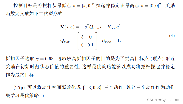
    def get_reward(self, x, u):
        """
        计算奖励信号
        """
        Q_rew = np.matrix([[5, 0], [0, 0.1]])
        R_rew = 1
        x_ = np.matrix(x)
        return -x_*Q_rew*x_.T - R_rew*(u**2)

然后是Qlearning算法，继承上面写的Pendulum

Q_learning.py

采用的是Q学习和epsilon贪心算法

import numpy as np
from matplotlib import pyplot as plt

from pendulum_env import Pendulum


class Q_learning(Pendulum):
    """
    Q学习，继承自己写的环境prndulum
    """

    def __init__(self, iterations=12000, gamma=0.98, lr=0.5):
        super().__init__()

        # 超参数
        # 迭代次数
        self.N = iterations
        # 折扣因子
        self.gamma = gamma
        # 学习率
        self.lr = lr

        # 常量
        # 动作矩阵
        self.actions = np.array([-3, 0, 3])
        # 初始状态
        self.inite_x = np.array([-np.pi, 0])
        # 控制误差 角度和角速度
        self.control = np.array([0.05, 0.01])
        # 探索步长限制
        self.step_control = 300

    def get_greedy_act(self, Q, x, epsilon):
        """
        epsilon贪心搜索策略
        :param Q: Q函数矩阵
        :param x: 状态空间
        :param epsilon: 贪心算法的参数ε
        :return: 贪心策略动作下标
        """
        opt_act = np.argmax(Q[:, x[0], x[1]])
        if np.random.random() > epsilon:
            return opt_act
        else:
            return np.random.choice([0, 1, 2])

    def train(self, num_alpha=200, num_d_alpha=200, epsilon=1.0, decay=0.9995):
        """
        训练学习
        :param num_alpha: 角度离散阶数
        :param num_d_alpha: 角速度离散阶数
        :param epsilon: 贪心算法的参数ε
        :param decay: 学习率更新参数
        :return: history
        """
        # 存储所有状态以及所有动作的Q函数矩阵
        Q = np.zeros([3, num_alpha, num_d_alpha])

        epsilon_limit = 0.01  # epsilon的下界
        lr = self.lr
        total_step = 0

        # 最优值记录
        optimal = -1e7      # 最优奖励
        finalerror = 2 * np.pi  # 最小误差

        reward_list = []

        history = {'avg rewards': [],
                   'avg steps': [],
                   'Q': [],
                   'locations': [],
                   'actions': []}

        # 开始迭代
        for i in range(self.N):
            x = self.inite_x
            count, total_reward = 0, 0

            sample_x = self.action_sample(x, num_alpha, num_d_alpha)
            epsilon = max(decay * epsilon, epsilon_limit)
            lr = decay * lr
            locations, total_acts = [], []

            locations.append(x[0])
            error_a = np.abs(x[0])
            while count < self.step_control:
                count += 1
                greedy_act = self.get_greedy_act(Q, sample_x, epsilon)
                next_act = self.actions[greedy_act]
                total_acts.append(next_act)

                # 计算reward
                reward = self.get_reward(x, next_act)

                # 计算下一个转移状态
                new_x = self.get_next_state(x, next_act)
                # 计算当前状态与目标状态的误差
                error_a = np.abs(new_x[0])
                # 如果满足目标就break
                if np.abs(new_x[0]) < self.control[0] and np.abs(new_x[1]) < self.control[1]:
                    locations.append(new_x[0])
                    break

                # 对新状态采样
                new_sample_x = self.action_sample(new_x, num_alpha, num_d_alpha)
                # 计算Q函数
                max_newQa = np.max(Q[:, new_sample_x[0], new_sample_x[1]])
                delta = reward + self.gamma * max_newQa - Q[greedy_act][sample_x[0]][sample_x[1]]
                Q[greedy_act][sample_x[0]][sample_x[1]] += lr * delta

                # 更新状态
                x, sample_x = new_x, new_sample_x
                locations.append(x[0])  # 记录下一个角度
                total_reward += reward  # 记录reward值
            reward_list.append(total_reward)
            avg_reward = np.mean(reward_list[-100:])

            total_step += count
            avg_step = total_step / 100

            # 历史记录
            history['avg rewards'].append(avg_reward)
            history['avg steps'].append(avg_step)
            history['Q'].append(Q)
            history['locations'].append(locations)
            history['actions'].append(total_acts)

            # 若该次迭代优于上次或奖励更高，则更新最佳值
            if count < self.step_control:
                # if error_a < finalerror or (error_a == finalerror and total_reward > optimal):
                if error_a < finalerror or total_reward > optimal:
                    optimal, finalerror = total_reward, error_a
            # 每100次打印信息
            if (i + 1) % 100 == 0:
                print("* Episode {}/{} ** Avg Step is ==> {} ** Avg Reward is ==> {} *".format(i + 1, self.N,
                                                                                               avg_step,
                                                                                               avg_reward))
                total_step = 0

        print("最终距离稳定状态角度误差为:%f rad" % np.abs(locations[-1]))
        return history

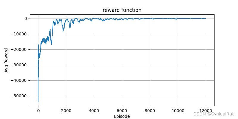
    def plot_reward(self, history, reward=True, step=True):
        """
        绘制历史信息
        :param history: 历史记录
        :param reward: 价值函数标志位
        :param step: 更新步长标志位
        :return:
        """
        if reward:
            plt.figure(figsize=(8, 4))
            plt.title("reward function")
            plt.plot(np.array(history['avg rewards']).reshape(-1))
            plt.xlabel("Episode")
            plt.ylabel("Avg Reward")
            plt.grid()
            plt.savefig('rewards.jpg')
            plt.show()

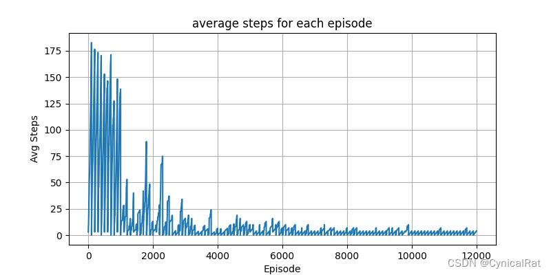
        if step:
            plt.figure(figsize=(8, 4))
            plt.title("average steps for each episode")
            plt.plot(np.array(history['avg steps']).reshape(-1))
            plt.xlabel("Episode")
            plt.ylabel("Avg Steps")
            plt.grid()
            plt.savefig('steps.jpg')
            plt.show()


q = Q_learning(iterations=12000, lr=0.5)
History = q.train(epsilon=0.5)
# print(History['avg rewards'])
q.plot_reward(History)
# print(History['actions'][:10])
# print(History['actions'][-10:])

最后的可视化结果

 

后面还会尝试实现SARSA、DQN等等算法，持续更新中....