StudyNote---Python For Data Analysis

准备工作

1. 安装Anaconda
2. 安装Jupyter notebook
3. 安装ipython

Python语法基础

1. 万物皆对象
2. 动态引用，强类型

isinstance(a, int)  #检查a是否为int实例 

3. 鸭子类型
4. 列表、字典、NumPy数组，和用户定义的类型（类），都是可变的；字符串和元组，是不可变的
5. 对于有换行的字符串，可以使用三引号，’’'或"""
6. 三元表达式

Python数据结构和序列

1. 元组

In [1]: tup = 4, 5, 6

2. tuple方法
3. 列表
4. 二级排序 b.sort(key=len)
5. bisect 二分搜索
6. 匿名函数

equiv_anon = lambda x: x * 2

7. 柯里化：部分参数应用
8. 生成器

NumPy基础

• NumPy是在一个连续的内存块中存储数据，独立于其他Python内置对象。NumPy的C语言编写的算法库可以操作内存，而不必进行类型检查或其它前期工作。比起Python的内置序列，NumPy数组使用的内存更少。
• NumPy可以在整个数组上执行复杂的计算，而不需要Python的for循环。

numpy使用

import numpy as np
# ndarray是一个通用的同构数据多维容器
#也就是说，其中的所有元素必须是相同类型的。每个数组都有一个shape（一个表示各维度大小的元组）
#和一个dtype（一个用于说明数组数据类型的对象
data1 = [6,7.5,8,0,1]
arr1 = np.array(data1)
arr1.shape
arr1.dtype
# 嵌套序列
data2 = [[1, 2, 3, 4], [5, 6, 7, 8]]
arr2 = np.array(data2)

numpy数组的运算

不用编写循环即可对数据执行批量运算。
NumPy用户称其为矢量化（vectorization）。
大小相等的数组之间的任何算术运算都会将运算应用到元素级

data = [[1.,2.,3.],[4.,5.,6.]]
arr = np.array(data)
arr+arr
arr*arr

基本的索引和切片

数组切片是原始数组的视图。这意味着数据不会被复制，视图上的任何修改都会直接反映到源数组上。

arr = np.arange(10)
#arr:[0,1,2,3,4,5,6,7,8,9]
arr_slice = arr[5:8]
arr_slice[1]=12345
#arr:[0,1,2,3,4,5,12345,7,8,9]

注意：如果想要得到ndarray切片的一份副本而非视图，
就需要明确地进行复制操作，例如arr[5:8].copy()。

切片索引

 arr2d = np.array([[1,2,3],[4,5,6],[7,8,9]])
 arr2d[:2,1:]
 #第一个表示对行切，第二个表示对列切。
 #切取0，1行。得到[[1,2,3],[4,5,6]]
 #再将得到的数组从1列开始切。得到
 # [[2,3],[5,6]]
 #“只有冒号”表示选取整个轴，因此你可以像下面这样只对高维轴进行切片：
 arr2d[:, :1]
 #array([[1],
   [4],
   [7]])

布尔型索引

In [98]: names = np.array(['Bob', 'Joe', 'Will', 'Bob', 'Will', 'Joe', 'Joe'])
In [99]: data = np.random.randn(7, 4)
In [102]: names == 'Bob'
Out[102]: array([ True, False, False,  True, False, False, False], dtype=bool)
In [103]: data[names == 'Bob']

花式索引

以特定顺序选取行子集，
只需传入一个用于指定顺序的整数列表或ndarray

In [117]: arr = np.empty((8, 4))
In [118]: for i in range(8):
   			arr[i] = i
In [120]: arr[[4, 3, 0, 6]]
Out[120]:
array([[ 4.,  4.,  4.,  4.],
       [ 3.,  3.,  3.,  3.],
       [ 0.,  0.,  0.,  0.],
       [ 6.,  6.,  6.,  6.]])

使用负数索引将会从末尾开始选取行
arr[[1, 5, 7, 2], [0, 3, 1, 2]]
选取的是(1,0)、(5,3)、(7,1)和(2,2)
arr[[1, 5, 7, 2]][ :, [0, 3, 1, 2]]
先选取1,5,7,2行。每一行再按照0，3，1，2排序

数组转置和轴对换

#转置
arr.T
#计算矩阵内积
np.dot(arr.T,arr)
#transpose需要得到一个由轴编号组成的元组才能对这些轴进行转置
arr.transpose((1,0,2)) #第一个轴被换成了第二个，第二个轴被换成了第一个，最后一个轴不变。
#swapaxes方法，它需要接受一对轴编号;swapaxes也是返回源数据的视图（不会进行任何复制操作）。

通用函数

对ndarray中的数据执行元素级运算的函数。
可看做简单函数（接受一个或多个标量值，并产生一个或多个标量值）的矢量化包装器。

#返回一个数组
np.sqrt(arr)
np.exp(arr)
np.maximum(x, y)
#返回多个数组
remainder, whole_part = np.modf(arr)
#Ufuncs可以接受一个out可选参数，这样就能在数组原地进行操作
np.sqrt(arr, arr)

其他函数见书

利用数组进行数据处理

用数组表达式代替循环的做法，通常被称为矢量化

np.meshgrid函数接受两个一维数组，并产生两个二维矩阵（对应于两个数组中所有的(x,y)对）
xs, ys = np.meshgrid(points, points)

将条件逻辑表述为数组运算

result = np.where(cond,x,y)
cond为一个条件数组，如果cond中为true,使用x替换，如果为false，使用y替换

数学和统计方法

arr.mean()
arr.mean(axis=1) #计算该轴（1）向上的统计值
arr.sum()
arr.sum(axis=0) #计算该轴（0）向上的统计值
arr.cumsum()
arr.cumsum(axis=0)
arr.cumprod()
arr.cumprod(axis=0)

排序

#就地排序
arr.sort()
arr.sort(0) #按列排序
arr.sort(1) #按行排序
# np.sort()返回数组的已排序副本
np.sort(arr)

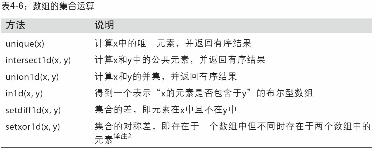
唯一化以及其他的集合逻辑

np.unique(names) #找出数组中的唯一值，并返回已排序的结果
np.in1d(values,array) #返回与values等长的布尔型数组，代表每个values数组中的值是否在array中

用于数组的文件输入输出

 np.save('some_array', arr)
 #将多个数组保存到一个未压缩文件中
 np.savez('array_archive.npz', a=arr, b=arr)
 #加载.npz文件
 arch = np.load('array_archive.npz')
 arch['b']
 #需要将数据压缩
 np.savez_compressed('arrays_compressed.npz', a=arr, b=arr)

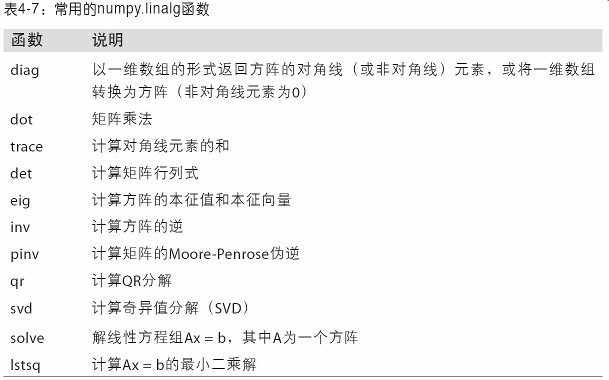
线性代数

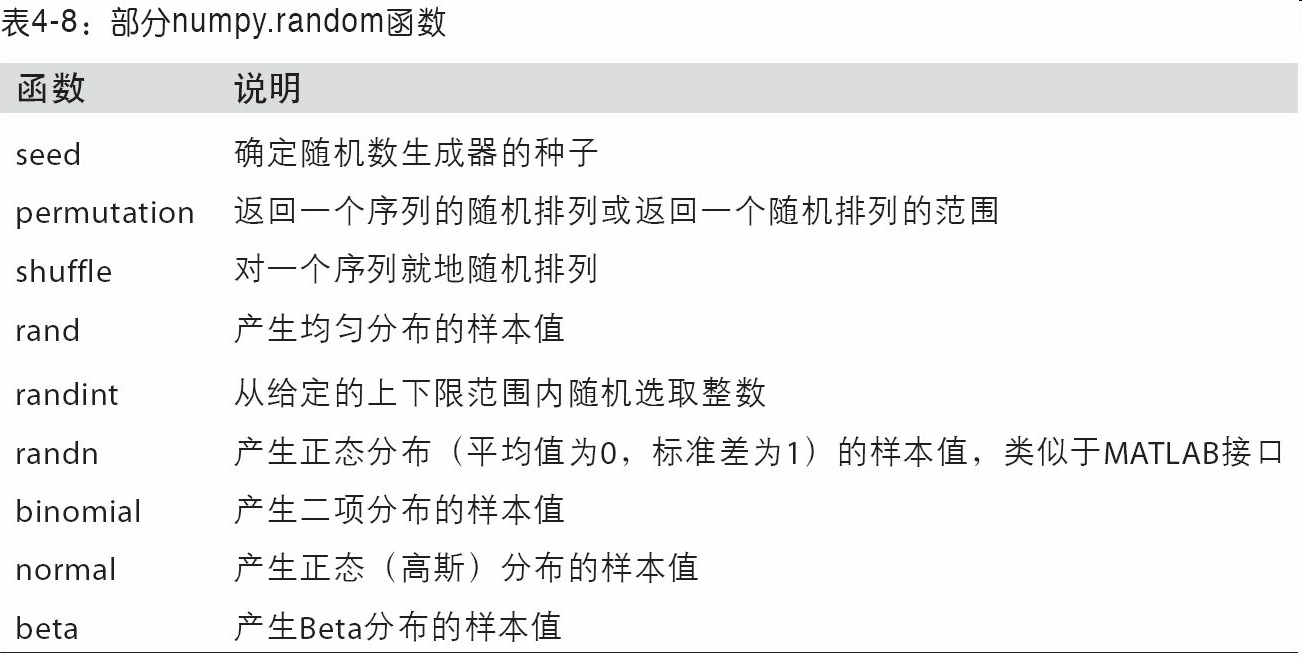
伪随机数生成

samples = np.random.normal(size=(4, 4))
rng = np.random.RandomState(1234) #避免全局状态

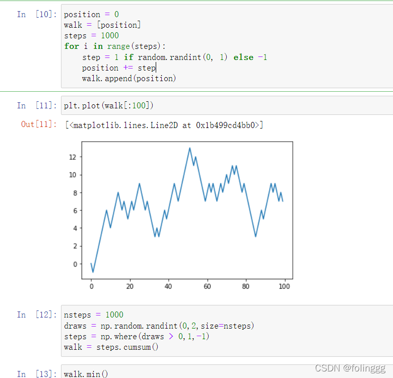
示例：随机漫步

pandas入门

Series

相当于一个Map

DataFrame

相当于一个表格

data = {’a':[1,2,3],'b':[4,5,6]}  #a,b相当于列的名称，每列有三个数
frame = np.DataFrame(data) 
frame = np.DataFrame(data，columns['b','a'],index=['one','two','three']) # 列按照b a 从左到右展示 ,行按照one,two,three从上到下展示
# 从DataFrame的列中获取一个Series 。 列可以进行赋值
frame['a']
frame.a
# 获取DataFrame的行
frame.loc['three']
# 对DataFrame进行赋值Series时，会精确匹配DataFrame的索引，空位填上缺失值
frame['a'] = pd.Series([3,4,5],index=['one','three','two'])
# del 可以删除列
del frame['a']
#嵌套字典

索引对象

将索引作为对象，进行存储。
索引对象不可修改，pandas的Index可以包含重复的标签。

index = obj.index
index[1] = 'b'   ❌
pd.index = (['a','a','b'])

基本功能

1. 重新索引 reindex

# 返回的是修改后的副本
obj.reindex(['a','c','b'])
obj.reindex(columns = ['ohio','texas','california'])
# 插值，使用ffill可以实现前向值填充
obj.reindex(range(6),method='ffill')
# 修改行和列名称时，已存在的行/列数据不变，原表格未存在的行/列数据为NaN

2. 丢弃指定轴上的项

# 返回的是修改后的副本
obj.drop(['d', 'c'])   # 删除行
data.drop('two', axis=1)   #删除列    axis代表轴，0代表横轴，1代表纵轴
# 就地修改
obj.drop('c', inplace=True)

3. 索引、选取和过滤

# 索引
obj = pd.Series(np.arange(4),index=['a','b','c','d'])
obj['a']
obj[1]
obj[:2]
obj[['a','b']]
obj[obj<2]
obj['a':'c'] #末端包含

4. loc和iloc

loc通过名字，iloc通过整数
data.loc['ohio']
data.loc[['ohio','utah']]    #选行
data.loc[:2,['one','three']]  #选择前两行的one，three列
data.iloc[0]
data.iloc[[0,2]]
data.iloc[:2,[0,2]]

5. 算术运算和数据对齐
   不包括的自动填充NaN

6. DataFrame和Series之间的运算

# 返回副本，广播形式
series = frame.iloc[0]
frame - series  # 将Series的索引匹配到DataFrame的列，然后沿着行一直向下广播
frame + series2 #  某个索引值在DataFrame的列或Series的索引中找不到，则参与运算的两个对象就会被重新索引以形成并集
series3 = frame['d']
frame.sub(series3, axis='index') #匹配行，且在列上广播  可axis=0

7. 函数应用和映射

# 常规
np.abs(frame)
# apply
f = lambda x: x.max() - x.min()
frame.apply(f)  # f是一个函数
# apply可以返回由多个值组成的Series
def f(x):
     return pd.Series([x.min(), x.max()], index=['min', 'max'])
frame.apply(f)  # f是一个函数
# applymap 应用于元素级别   （每个数据保留两位小数）
format = lambda x: '%.2f' % x
frame.applymap(format)

8. 排序和排名

# 返回副本
frame.sort_index()
frame.sort_index(axis=1, ascending=False) # 括号中内容选填  此代表按列降序排序
frame.sort_values(by=['b','a'])  # 根据一个或多个列中的值进行排序
frame.rank(axis='columns')  # 在列上计算排名

series.sort_values() # 按值排序  NaN值默认放到series末尾
series.rank() # rank是通过“为各组分配一个平均排名”的方式破坏平级关系
series.rank(method='first') # 根据值在原数据中出现的顺序给出排名：

9. 带有重复标签的轴索引

obj = pd.Series(range(4),index=['a','a','b','c'])
obj['a']   # 返回Series   
obj['b']   # 返回标量
obj.index.is_unique # 返回轴是否重复

汇总和计算描述统计

1. 常规

axis = 0 列
axis = 1 行
df.sum() # 自动排除NaN值   skipna=False 可以取消该功能
df.mean()
df.idxmax()
df.cumsum()
df.describe()  # 一次性产生多个汇总统计
#更多方法查看书

2. 相关系数与协方差

更改axis='columns’ 可以按照行进行计算
returns = price.pct_change() # 计算百分数变换
returns.tail()
returns['MSFT'].corr(returns['IBM']) # corr方法用于计算两个Series中重叠的、非NA的、按索引对齐的值的相关系数
returns['MSFT'].cov(returns['IBM']) # cov用于计算协方差
returns.corrwith(returns.IBM) # 计算其列或行跟另一个Series或DataFrame之间的相关系数
 

3. 唯一值、值计数以及成员资格

uniques = obj.unique() # 得到Series中的唯一值数组：
obj.value_counts() # 计算一个Series中各值出现的频率
pd.value_counts(obj.values, sort=False) # value_counts还是一个顶级pandas方法，可用于任何数组或序列
mask = obj.isin(['b', 'c']) # 判断矢量化集合的成员资格
pd.Index(unique_vals).get_indexer(to_match) # 可以给你一个索引数组，从可能包含重复值的数组到另一个不同值的数组
result = data.apply(pd.value_counts).fillna(0)

数据加载、存储与文件格式

读取文本格式的数据

# 常规
pd.read_csv('examples/ex1.csv')	#自动将第一行作为header, 默认分隔符为逗号
pd.read_csv('examples/ex1.csv',header=None) # 列使用默认0，1，2，3....
pd.read_csv('examples/ex1.csv',names=['a','b','c']) # 指定列名
pd.read_csv('examples/ex1.csv', names=names, index_col='message') #指定message列为索引
parsed = pd.read_csv('examples/ex1.csv',index_col=['key1', 'key2'])# 多个列做成一个层次化索引
pd.read_csv('examples/ex4.csv', skiprows=[0, 2, 3]) #用skiprows跳过文件的第一行、第三行和第四行
pd.isnull(parsed)
sentinels = {'message': ['foo', 'NA'], 'something': ['two']}
pd.read_csv('examples/ex5.csv', na_values=sentinels) # 字典的各列可以使用不同的NA标记值

pd.read_table('ex1.csv') # 默认分隔符为'\t'
pd.read_table('ex1.csv',sep=',') # 指定分隔符','

逐块读取文本文件

pd.read_csv('examples/ex6.csv',nrows = 5) #读取前五行
# 根据chunksize对文件进行逐块迭代
chunker = pd.read_csv('examples/ex6.csv',chunksize=1000) 
tot = pd.Series([])
for piece in chunker:
    tot = tot.add(piece['key'].value_counts(), fill_value=0)
tot = tot.sort_values(ascending=False)

将数据写出到文本格式

data.to_csv('examples/out.csv') # 写入到一个以逗号分割的文件中，(文件中第一个字符为逗号）
data.to_csv('examples/out.csv',sep='|') # 写入到以| 为分隔符的文件中

处理分隔符格式

import csv
f = open('examples/ex7.csv')    # open是打开文件函数，f此时是一个文件对象
reader = csv.reader(f) # reader按行存储
for line in reader:
	print(line) 		# 对reader进行迭代，为每行产生一个元组

剩下的不太懂，记下

JSON 数据

# Json-->对象
result = json.loads(jsonObj)
result['a'] 获取Json属性为a 的那个
siblings = pd.DataFrame(result['siblings'], columns=['name', 'age']) # 传入result['xx'] 
# 特别格式的JSON数据集 会自动转换
data = pd.read_json('examples/example.json')
# 对象-->Json
jsonObj = json.dumps(result)

XML和HTML

主要下载lxml和beautifulsoup4和html5lib

conda install lxml
pip install beautifulsoup4 html5lib

利用lxml.objectify解析XML

用lxml.objectify解析文件，然后通过getroot得到该XML文件的根节点的引用
不是很懂，记下此处。

path = 'datasets/mta_perf/Performance_MNR.xml'
parsed = objectify.parse(open(path))
root = parsed.getroot()

二进制数据格式

frame.to_pickle('examples/frame_pickle') # 以pickle格式保存到磁盘上
pd.read_pickle('examples/frame_pickle') # 读取被pickle化的数据
# pickle仅建议用于短期存储格式

HDF5格式

# 存储到mydata.h5
store = pd.HDFStore('mydata.h5')
store['obj1'] = frame
store['obj1_col'] = frame['a']
store
# HDF5对象的获取
store['obj1']
# 查询
store.put('obj2', frame, format='table')
store.select('obj2', where=['index >= 10 and index <= 15'])

读取Microsoft Excel文件

# 创建路径
xlsx = pd.ExcelFile('examples/ex1.xlsx')
# 读取excel文件
pd.read_excel(xlsx, 'Sheet1')
frame = pd.read_excel('examples/ex1.xlsx', 'Sheet1') # 等价

# 写成excel格式
# 创建ExcelWriter
writer = pd.ExcelWriter('examples/ex2.xlsx')
# to_excel方法
frame.to_excel(writer, 'Sheet1')
writer.save()
# 以下等价
frame.to_excel('examples/ex2.xlsx')

Web APIs交互

resp = requests.get(url)
# 响应对象的json方法会返回一个包含被解析过的JSON字典
data = resp.json()
data[0]['title']   # 显示data 0行 title 列 对应的数据
# 提取感兴趣的字段
issues = pd.DataFrame(data, columns=['number', 'title','labels', 'state'])

数据库交互

con = sqlite3.connect('mydata.sqlite')
con.execute(query)
# 插入数据
data = [('Atlanta', 'Georgia', 1.25, 6),('Tallahassee', 'Florida', 2.6, 3),('Sacramento', 'California', 1.7, 5)]
stmt = "INSERT INTO test VALUES(?, ?, ?, ?)"
con.executemany(stmt,data)
# 返回元组列表
cursor = con.execute('select * from test')
rows = cursor.fetchall()
pd.DataFrame(rows, columns=[x[0] for x in cursor.description])
# sqlalchemy
db = sqla.create_engine('sqlite:///mydata.sqlite')
pd.read_sql('select * from test', db)

数据清洗和准备

滤除缺失数据

df.dropna() # 默认删除含有NA的行
df.dropna(axis = 1) # 默认删除含有NA的列
df.dropna(thresh = 2) # 只想留下一部分观测数据

填充缺失数据

df.fillna(0)	# 使用0进行填充
df.fillna({1:0.5,2:0})	# 特定列填充特定数
df.fillna(0,inplace = True)	# 就地
df.fillna(method='ffill') # 使用前向值填充
df.fillna(method='ffill', limit=2) #  （对于前向和后向填充）可以连续填充的最大数量

移除重复数据

data.duplicated() # 返回一个布尔型Series，表示各行是否是重复行（前面出现过的行）
data.drop_duplicates() # 将重复的行丢掉 
data.drop_duplicates(['l1']) # 将k1列中重复的数据所在行丢掉
data.drop_duolicates(['k1','k2'],keep='last') # 保留最后一个（默认保留第一个）

利用函数或映射进行数据转换

# 大小写转变
lowercased = data['food'].str.lower() # 将food列转换为小写
# 映射
meat_to_animal = {
  'bacon': 'pig',
  'pulled pork': 'pig',
  'pastrami': 'cow',
}
data['animal'] = lowercased.map(meat_to_animal) # 将meat_to_animal与animal列相对应
          food  ounces  animal
0        bacon     4.0     pig
1  pulled pork     3.0     pig
2        bacon    12.0     pig
3     Pastrami     6.0     cow
# 一个函数完成工作:
data['food'].map(lambda x: meat_to_animal[x.lower()])

替换值

data.replace([x1,x2],[y1,y2]) # 使用y1,y2来替换x1,x2
data.replace({x1:y1,x2:y2}) # 同上

重命名轴索引

# 使用map方法
transform = lambda x: x[:4].upper()
data.index.map(transform)    # map方法 返回副本
# 使用rename方法
data.rename(index=str.title, columns=str.upper)
# 部分轴标签更新
data.rename(index={'OHIO': 'INDIANA'},columns={'three': 'peekaboo'})
# 就地修改，添加inplace = True

离散化和面元划分

# cut
# 将一组ages划分为不同的组(bins)
bins = [18,25,35,60,100] # 代表划分的标准，(18,25]  （25，35]   (35,60] ....
cats = pd.cut(ages,bins) # 划分ages    添加right = False 可以变成[ , )
cats = pd.cut(ages, bins, labels=group_names) # 设置自己的面元名称
cats = pd.cut(data,4,precision = 2)   # 等长面元，划分成成4组，单个数据限定2位小数。
# cats.codes（每个age对应于哪个区间的下标）    cats.categories（代表每个组名称）
# qcut 根据样本分位数对数据进行面元划分 得到大小基本相等的面元
cats = pd.qcut(data, 4)  # Cut into quartiles
pd.qcut(data, [0, 0.1, 0.5, 0.9, 1.]) # 传递自定义的分位数（0到1之间的数值，包含端点)

检测和过滤异常值

col[np.abs(col) > 3] # 通过数组运算进行检测和过滤异常值
data[(np.abs(data) > 3).any(1)] # 选出全部含有“超过3或－3的值”的行

排列和随机采样

sampler = np.random.permutation(5) # 产生一个随机的排列顺序
df.take(sampler)	# 根据sampler值，进行行的排序
# sample方法
df.sample(n=3)	# 直接对df行进行随机选取，n的值代表选取出来的行数量
draws = choices.sample(n=10, replace=True) # 替换的方式产生样本（允许重复选择）

计算指标/哑变量

一个电影可以属于好几种类别，如果把不同类别作为列，每个电影所属类别对应列里面打1。这样应该怎么做呢？

# 将一列里面重复的不同值，作为不重复的单个列名。
pd.get_dummies(df['key']) #某一列中含有k个不同的值，则可以派生出一个k列矩阵或DataFrame（其值全为1和0）
dummies = pd.get_dummies(df['key'], prefix='key') # 这里就是在列名上加一个前缀
# 电影例子：
假设电影是movies
movies = pd.read_table('datasets/movielens/movies.dat', sep='::',header=None, names=mnames)
# 首先得得到类别
all_genres = []
for x in movies.genres:
    all_genres.extend(x.split('|'))
genres = pd.unique(all_genres)
# 然后这个时候可以构造一个全零的DataFrame，用于存放对应关系
zero_matrix = np.zeros((len(movies), len(genres)))
dummies = pd.DataFrame(zero_matrix, columns=genres)
# 迭代每一部电影，并在dummies中设置值
for i, gen in enumerate(movies.genres):
    indices = dummies.columns.get_indexer(gen.split('|'))
    dummies.iloc[i, indices] = 1
# 和原来的合并
movies_windic = movies.join(dummies.add_prefix('Genre_'))

字符串操作

都是一些基本操作啦，基本一看就知道是啥

# 分割/连接
val.split(',')
# 这个strip是用来去除空白符的，包括换行符
pieces = [x.strip() for x in val.split(',')] 
first, second, third = pieces
first + '::' + second + '::' + third
'::'.join(pieces)
# 查看
'guido' in val
val.index(',') # 找不到引发异常
val.find(':')  # 找不到返回-1
val.count(',')
# 更改
val.replace(',', '::')

正则表达式

简单举几个

re.split('\s+', text)
regex.findall(text)
regex.search(text)
regex.match(text)
regex.sub('REDACTED', text)

pandas的矢量化字符串函数

字典没有isnull()方法，所以先转换成Series

data = pd.Series(data)
data.isnull()
# 可以查看是否包含某个字符串
data.str.contains('gmail') 
# 也可以使用正则表达式，还可以加上任意re选项(如IGNORECASE) 
matches = data.str.findall(pattern, flags=re.IGNORECASE)
# 矢量化元素的获取操作
# str.get
matches.str.get(1)
# 在str属性上使用索引
matches.str[0]
# 截取
data.str[:5]

数据规整：聚合、合并和重塑

层次化索引

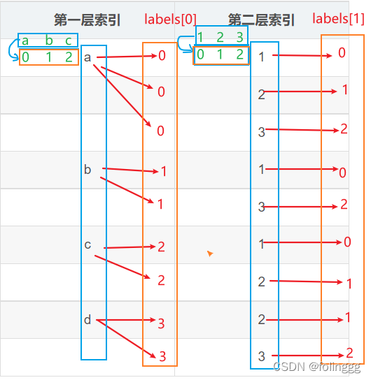
MultiIndex 代表多层索引

MultiIndex(levels=[['a', 'b', 'c', 'd'], [1, 2, 3]],
           labels=[[0, 0, 0, 1, 1, 2, 2, 3, 3], [0, 1, 2, 0, 2, 0, 1, 1, 2]])

以上为例，levels代表每层的索引

第一层索引	第二层索引
a	1
	2
	3
b	1
	3
c	1
	2
d	2
	3

MultiIndex的labels其中的数组代表在第某层索引中处于的位置。
一共十个数，前三个数属于a,故labels的第一个元组前三个为0，0，0。四五属于b，故labels的第一个元组第四五个为1,1。labels第二个元组同理。

对于Series

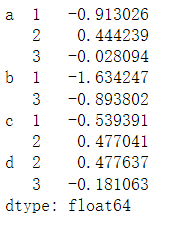
# Series是选取行
data['b':'d']
data['b','d']
data.loc[:,1]    # 注意这里的1指的是索引的名称，而不是索引下标
data.unstack()   # 变为DataFrame
data.unstack().stack() # 逆运算

对于DataFrame

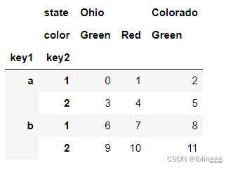
# DataFrame是选取列
frame['Ohio']
# 可以指定index和columns的名字
frame.index.names = ['key1', 'key2']
frame.columns.names = ['state', 'color']

重排与分级排序

为了调整某条轴上各级别的顺序，但数据不会发生变化。

frame.swaplevel('key1', 'key2')

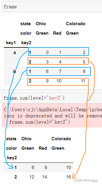
根据级别汇总统计

使用DataFrame的列进行索引

frame2 = frame.set_index(['c', 'd'])

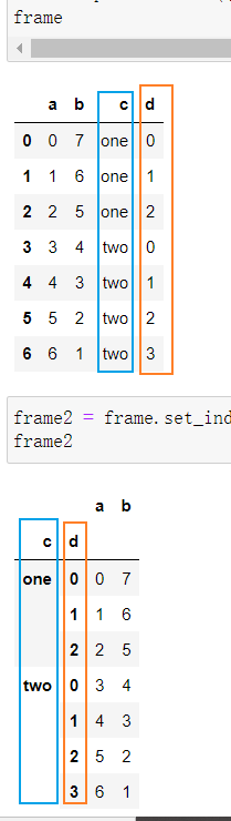
# 默认情况下，那些列会从DataFrame中移除，但也可以将其保留下来
frame.set_index(['c', 'd'], drop=False)
# reset_index的功能跟set_index刚好相反，层次化索引的级别会被转移到列里面
frame2.reset_index()

合并数据集

轴向连接

合并重叠数据

重叠数据保留前面的

对于Series
b.combine_first(a)
对于DataFrame
df1.combine_first(df2)

重塑和轴向旋转

1. 重塑层次化索引
   
   unstack 逆过程 如果找不到值，使用NaN，stack时也会滤除NaN
2. 将“长格式”旋转为“宽格式”
   没看太懂，记下

---

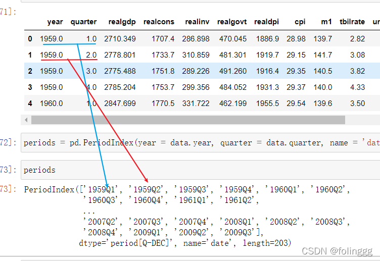
时间格式转换

periods = pd.PeriodIndex(year = data.year, quarter = data.quarter, name = 'date')

pivot进行行转列
pivoted = ldata.pivot('date', 'item', 'value')
前两个传递的值分别用作行和列索引，最后一个可选值则是用于填充DataFrame的数据列

将宽格式旋转为长格式

旋转DataFrame的逆运算是pandas.melt
合并多个列成为一个，产生一个比输入长的DataFrame

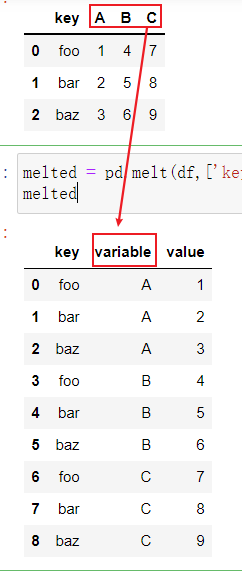
使用pivot，可以重塑回原来的样子

reshaped = melted.pivot('key', 'variable', 'value')

绘图和可视化

数据聚合与分组运算

groupby
想要按key1进行分组，并计算data1列的平均值

grouped = df['data1'].groupby(df['key1'])
返回的grouped只是一个GroupBy对象，还没进行任何计算。
是含有一些有关分组键df['key1']的中间数据。
# 计算平均值
grouped.mean()

# GroupBy的size方法，可以返回一个含有分组大小的Series
df.groupby(['key1', 'key2']).size()

对分组进行迭代

# name  代表根据key1分组的各个值
# group 代表各个分组具体的数据内容
for name, group in df.groupby('key1'):
   ....:     print(name)
   ....:     print(group)
# 多重键的情况
for (k1, k2), group in df.groupby(['key1', 'key2']):
   ....:     print((k1, k2))
   ....:     print(group)

选取一列或列的子集

因为groupby返回的是一个DataFrameGroupBy对象啦~（可以想成是一个DataFrame）所以可以取分组之后的某个列

df.groupby('key1')['data1']
df.groupby('key1')[['data2']]

通过字典或Series进行分组

数据聚合与分组运算

时间序列

pandas高级应用

Python建模库介绍

数据分析案例