


【Python · Pytorch】人工神经网络 ANN(下)
9. 应用实例
ANN / CNN 绘制网站:http://alexlenail.me/NN-SVG/index.html
常用Python库包含数据集:
-
torchvision
torchvision.datasets这个包本身并不包含数据集的文件本身,它的工作方式是先从网络上把数据集下载到用户指定目录,然后再用它的加载器把数据集加载到内存中。最后,将加载后的数据集作为对象返回给用户。
名称 说明 类型 维度 MNIST 手写数字 分类 28*28 EMNIST 手写字符 分类 28*28 Fashion-MNIST 服饰图标 分类 28*28 ImageNet 物体识别(21,841类) 分类 224*224 CIFAR-10 / CIFAR-100 物体识别 分类 32*32 Caltech 101 / Caltech 256 物体识别 分类 300*200 KITTI 自动驾驶视觉场景 分类 - SVHN 谷歌街景门牌号码 分类 - COCO 目标识别 分类 - PASCAL VOC 物体识别 分类 - …… …… …… …… -
scikit-learn
sklearn除load系列经典数据集外,还支持自定义数据集make系列和下载数据集fetch系列(load系列为安装sklearn库时自带,而fetch则需额外下载),这为更多的学习任务场景提供了便利。
名称 说明 类型 维度 load_boston Boston房屋价格 回归 506*13 fetch_california_housing 加州住房 回归 20640*9 load_diabetes 糖尿病 回归 442*10 load_digits 手写字 分类 1797*64 load_iris 鸢尾花 分类 / 聚类 (50*3)*4 load_wine 葡萄酒 分类 (59+71+48)*13 load_linnerud 体能训练 多分类 20 …… …… …… …… -
其他常见数据集
名称 说明 类型 维度 FDDB / LFW 人脸识别 分类 - WiderPerson 密集行人检测 分类 - …… …… …… ……
9.1 分类
(1) 数据集介绍
IRIS鸢尾花数据集
IRIS鸢尾花数据集是常用的分类实验数据集,由Fisher于1936年收集。Iris也称鸢尾花卉数据集,属多重变量分析数据集。
数据集包含150个数据样本,分为3类,每类50个数据,每个数据包含4个属性。
| 序号 | 属性 | 单位 |
|---|---|---|
| 1 | Sepal.Length(花萼长度) | cm |
| 2 | Sepal.Width(花萼宽度) | cm |
| 3 | Petal.Length(花瓣长度) | cm |
| 4 | Petal.Width(花瓣宽度) | cm |
种类:Iris Setosa(山鸢尾)、Iris Versicolour(杂色鸢尾)、Iris Virginica(维吉尼亚鸢尾)。
from sklearn.datasets import load_iris
(2) 训练模型
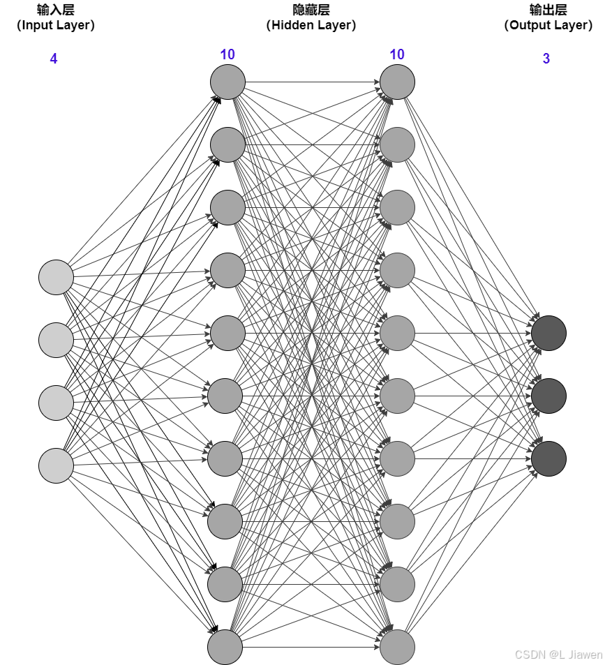
本小节将构建并训练人工神经网络,实现通过4个属性判断鸢尾花种类。
绘制网络结构图
① 导入三方库
import torch
import torch.nn as nn
import torch.nn.functional as F
import numpy as np
② 读取数据集
# Scikit-learn
from sklearn.datasets import load_iris
from sklearn.model_selection import train_test_split
from sklearn.neighbors import KNeighborsClassifier

data = load_iris()

X = data.data
y = data.target
划分数据集
X_train, X_test, y_train, y_test = train_test_split(X, y, random_state=12, stratify=y,test_size=0.3)
# Sepal: Length & Width
# Petal: Length & Width
# ## Setosa、Versicolour、Virginica

y_train_onehot = []

for i in range(len(y_train)):
    y = [0 for i in range(3)]
    y[y_train[i]] = 1
    y_train_onehot.append(y)
X_train = torch.Tensor(X_train)
X_test = torch.Tensor(X_test)
y_train = torch.Tensor(y_train_onehot)
y_test = torch.Tensor(y_test)
③ 创建人工神经网络
class ANN(nn.Module):
    n_input = 4
    n_h1 = 10
    n_h2 = 10
    n_output = 3

    def __init__(self):
        super(ANN, self).__init__()

        self.layers = nn.Sequential(
            nn.Linear(self.n_input, self.n_h1),
            nn.ReLU(),
            nn.Linear(self.n_h1, self.n_h2),
            nn.ReLU(),
            nn.Linear(self.n_h2, self.n_output),
        )

    def forward(self, x):
        return self.layers(x)
④ 训练人工神经网络
# 设置随机种子,保证初始化参数一致
torch.manual_seed(20)
# 创建模型对象
model = ANN()
# 定义损失函数
loss_function = nn.CrossEntropyLoss()
# 定义优化器
optimizer = torch.optim.Adam(model.parameters(), lr=0.01)
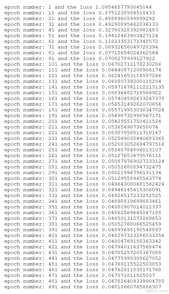
# 定义轮次
epochs = 500
# 累计损失
final_losses = []
for i in range(epochs):
# 1. 正向传播
y_pred = model(X_train)
# 2. 计算损失
loss = loss_function(y_pred, y_train)
final_losses.append(loss)
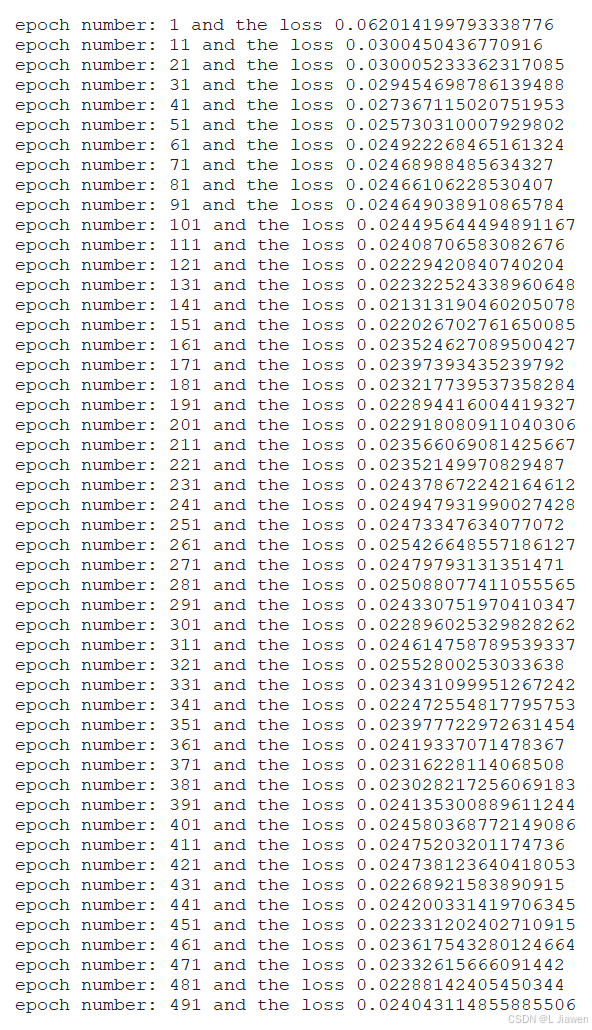
if i % 10 == 0:
print("epoch number: {} and the loss {}".format(i+1, loss.item()))
# 另一种写法:print("epoch number: %s and the loss %s"%(i+1, loss.item()))
# 清空梯度
optimizer.zero_grad()
# 3. 反向传播
loss.backward()
# 4. 优化参数
optimizer.step()
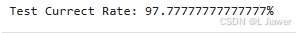
⑤ 测试人工神经网络
total = len(X_test)
currect = 0
with torch.no_grad():
    for i in range(total):
        outputs = model(X_test[i])
        _, predicted = torch.max(outputs.data, 0)
        if y_test[i] == predicted:
            currect += 1
print('Test Currect Rate: {}%'.format(currect / total * 100))
9.2 图像识别
9.2.1 手写数字识别
(1) 数据集介绍
Mnist数据集
手写数字识别数据集,数据集分为训练集和测试集,用于训练和评估机器学习模型。
该数据集在深度学习领域具有重要地位,尤其适合初学者学习和实践图像识别技术。
- 该数据集含有
10种类别,共70000个灰度图像。包含60000个训练集样本, 和10000个测试集样本。 - 每张图像以
28x28像素的分辨率提供。
# torchvision
import torch
import torchvision.datasets as dataset
import torchvision.transforms as transforms

# 读取训练集
train_data = dataset.MNIST(root = "mnist",
                           train = True,
                           transform = transforms.ToTensor(),
                           download = True)

# 读取测试集
test_data = dataset.MNIST(root = "mnist",
                           train = False,
                           transform = transforms.ToTensor(),
                           download = True)
(2) 训练模型
本小节将构建并训练人工神经网络,实现通过手写数字图片判断数字。
① 导入三方库
import os
import cv2
import torch
import torch.nn as nn
import numpy as np
import matplotlib.pyplot as plt
② 读取数据集
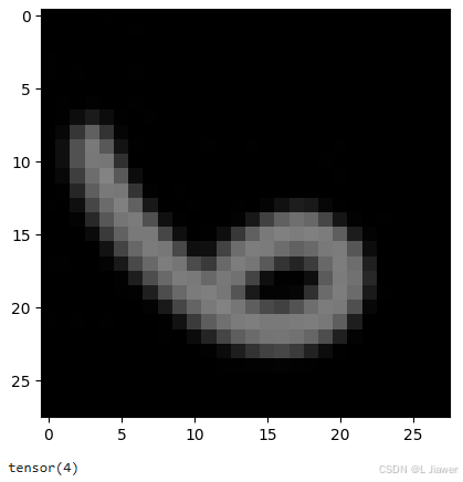
查看图片样例
""" 利用cv2查看 """
# img_demo = cv2.imread('./data/mnist/mnist_train_jpg_60000/0_5.jpg',cv2.IMREAD_GRAYSCALE)
# cv2.imshow('Image', img_demo)
# cv2.waitKey(0)
# cv2.destroyAllWindows()
""" 利用matplotlib.pyplot查看 """
img_demo = cv2.imread('./data/mnist/mnist_train_jpg_60000/0_5.jpg',cv2.IMREAD_GRAYSCALE)
plt.imshow(img_demo, cmap='gray', vmin=0, vmax=255)
plt.show()
读取训练集
""" 训练集 """
count = 0
X_train = []
y_train = []
train_path = './data/mnist/mnist_train_jpg_60000/'
for filename in os.listdir(train_path):
    filepath = os.path.join(train_path, filename)
    img = cv2.imread(filepath,cv2.IMREAD_GRAYSCALE)
    img = img.reshape(-1)
    X_train.append(img)
    y = np.zeros(10)
    y[int(filename.split('_')[1][0])] = 1
    y_train.append(y)

X_train = torch.Tensor(np.array(X_train))
y_train = torch.Tensor(np.array(y_train))
X_train.shape, y_train.shape
读取测试集
""" 测试集 """
# 测试集
X_test = []
y_test = []
y_test_num = []
test_path = './data/mnist/mnist_test_jpg_10000/'
for filename in os.listdir(test_path):
    filepath = os.path.join(test_path, filename)
    img = cv2.imread(filepath,cv2.IMREAD_GRAYSCALE)
    img = img.reshape(-1)
    X_test.append(img)
    y = np.zeros(10)
    y[int(filename.split('_')[1][0])] = 1
    y_test.append(y)

X_test = torch.Tensor(np.array(X_test))
y_test = torch.Tensor(np.array(y_test))
X_test.shape, y_test.shape
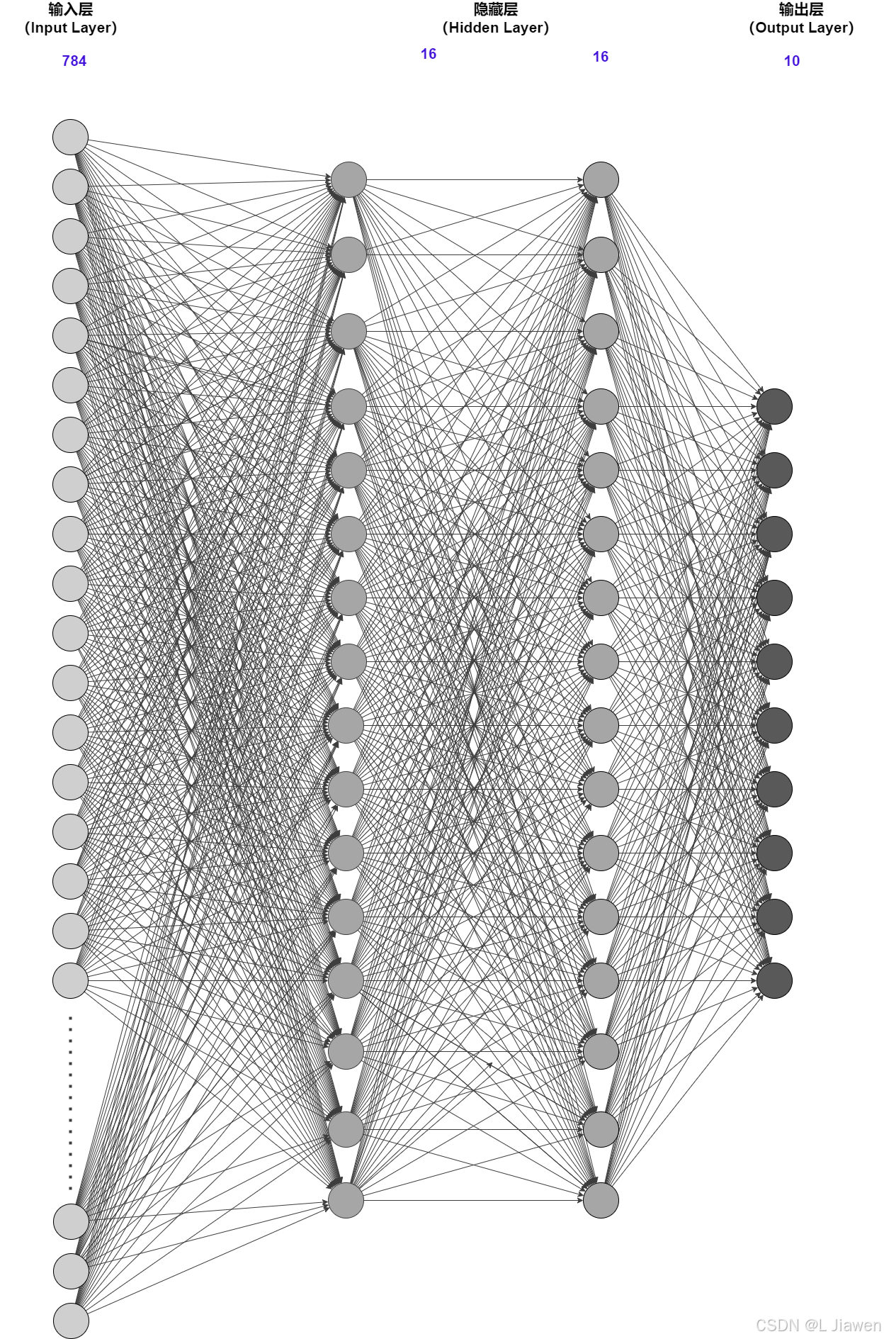
③ 创建人工神经网络
class ANN(nn.Module):
    n_input = 28*28
    n_h1 = 16
    n_h2 = 16
    n_output = 10

    def __init__(self):
        super(ANN, self).__init__()

        self.layers = nn.Sequential(
            nn.Flatten(),
            nn.Linear(self.n_input, self.n_h1),
            nn.ReLU(),
            nn.Linear(self.n_h1, self.n_h2),
            nn.ReLU(),
            nn.Linear(self.n_h2, self.n_output),
        )

    def forward(self, x):
        return self.layers(x)
④ 训练人工神经网络
torch.manual_seed(20)
model = ANN()
loss_function = nn.CrossEntropyLoss()
optimizer = torch.optim.Adam(model.parameters(), lr=0.01)
epochs = 500

final_losses = []
for i in range(epochs):
    # 1. 正向传播
    y_pred = model.forward(X_train)

    # 2. 计算loss
    loss = loss_function(y_pred, y_train)
    final_losses.append(loss)
    if i % 10 == 0:
        print("epoch number: {} and the loss {}".format(i+1, loss.item()))

    # 清空梯度
    optimizer.zero_grad()

    # 3. 反向传播
    loss.backward()
    # 4. 优化参数
    optimizer.step()
losses = [x.detach().numpy() for x in final_losses]
plt.plot(range(epochs), losses)
plt.ylabel('Loss')
plt.xlabel('Epoch')
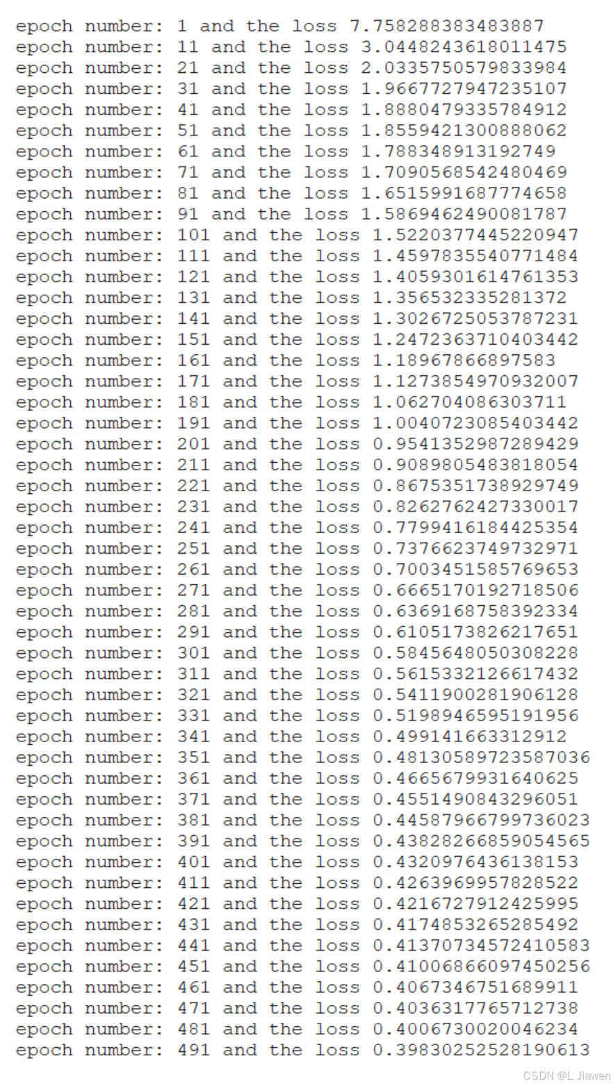
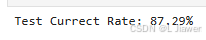
⑤ 测试人工神经网络
total = len(X_test)
currect = 0
with torch.no_grad():
    for i in range(total):
        outputs = model.forward(X_test[i])
        _, predicted = torch.max(outputs.data, 0)

        if y_test[i][predicted] == 1:
            currect += 1
print('Test Currect Rate: {}%'.format(currect / total * 100))
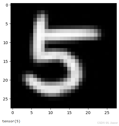
※ 提供人工手写案例
# res = 5
img_test = cv2.imread('./data/demo_5.jpg', cv2.IMREAD_GRAYSCALE)
plt.imshow(img_test, cmap='gray', vmin=0, vmax=255)
plt.show()
img_test = torch.Tensor(img_test.reshape(-1))

outputs = model(img_test)
_, predicted = torch.max(outputs.data, 0)
print(predicted)
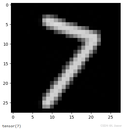
# res = 7
img_test = cv2.imread('./data/demo_7.jpg', cv2.IMREAD_GRAYSCALE)
plt.imshow(img_test, cmap='gray', vmin=0, vmax=255)
plt.show()
img_test = torch.Tensor(img_test.reshape(-1))

outputs = model(img_test)
_, predicted = torch.max(outputs.data, 0)
print(predicted)
这种神经网络对旋转数字抗性较差(虽然手写数字中6和9不适合旋转处理,但旋转角度不大,人类可以识别出6)
# res = 6 ×××
img_test = cv2.imread('./data/demo_6.jpg', cv2.IMREAD_GRAYSCALE)
plt.imshow(img_test, cmap='gray', vmin=0, vmax=255)
plt.show()
img_test = torch.Tensor(img_test.reshape(-1))

outputs = model(img_test)
_, predicted = torch.max(outputs.data, 0)
print(predicted)
9.2.2 衣物图标识别
(1) 数据集介绍
Fashion-Mnist数据集
衣物分类数据集,经典MNIST手写数字数据集的现代替代品的数据集。
- 该数据集含有
10种类别,共70000个灰度图像。包含60000个训练集样本, 和10000个测试集样本。 - 每张图像以
28x28像素的分辨率提供。

FashionMNIST包含以下10个类别:
- T-shirt/top (T恤/上衣)
- Trouser (裤子)
- Pullover (套头衫)
- Dress (连衣裙)
- Coat (外套)
- Sandal (凉鞋)
- Shirt (衬衫)
- Sneaker (运动鞋)
- Bag (包包)
- Ankle boot (踝靴)
# torchvision.datasets.FashionMNIST
(2) 训练模型
本小节将构建并训练人工神经网络,实现通过衣服图片判断衣服种类。
① 导入三方库
import torch
import torch.nn as nn
import numpy as np
② 读取数据集
torchvision读取
""" torchvision """
# import torch
# from torch import nn
# from torch.utils.data import DataLoader
# from torchvision import datasets
# from torchvision.transforms import ToTensor

# # Download training data from open datasets.
# training_data = datasets.FashionMNIST(
#     root="data",
#     train=True,
#     download=True,
#     transform=ToTensor(),
# )

# # Download test data from open datasets.
# test_data = datasets.FashionMNIST(
#     root="data",
#     train=False,
#     download=True,
#     transform=ToTensor(),
# )
文件读取
def load_mnist(path, kind='train'):
    import os
    import gzip
    import numpy as np

    """Load MNIST data from `path`"""
    labels_path = os.path.join(path, '{}-labels-idx1-ubyte.gz'.format(kind))
    images_path = os.path.join(path, '{}-images-idx3-ubyte.gz'.format(kind))

    with gzip.open(labels_path, 'rb') as lbpath:
        labels = np.frombuffer(lbpath.read(), dtype=np.uint8, offset=8)
    with gzip.open(images_path, 'rb') as imgpath:
        images = np.frombuffer(imgpath.read(), dtype=np.uint8, offset=16).reshape(len(labels), 28*28)

    return images, labels
读取数据集
X_train, y_train = load_mnist(path='./data/fashion-mnist/')
X_test, y_test = load_mnist(path='./data/fashion-mnist/', kind='t10k')

y_train_onehot = []

for i in range(len(y_train)):
    y = [0 for i in range(10)]
    y[y_train[i]] = 1
    y_train_onehot.append(y)

y_train = y_train_onehot
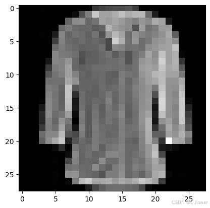
图片数据输出
import matplotlib.pyplot as plt

plt.imshow(X_test[4].reshape(28,28), cmap='gray', vmin=0, vmax=255)
plt.show()
③ 创建人工神经网络
class ANN(nn.Module):
    n_input = 784
    n_h1 = 512
    n_h2 = 256
    n_h3 = 128
    n_h4 = 64
    n_h5 = 32
    n_h6 = 10
    n_output = 10

    def __init__(self):
        super(ANN, self).__init__()

        self.layers = nn.Sequential(
            nn.Linear(self.n_input, self.n_h1),
            nn.ReLU(),
            nn.Dropout(0.2),
            nn.Linear(self.n_h1, self.n_h2),
            nn.ReLU(),
            nn.Dropout(0.2),
            nn.Linear(self.n_h2, self.n_h3),
            nn.ReLU(),
            nn.Dropout(0.2),
            nn.Linear(self.n_h3, self.n_h4),
            nn.ReLU(),
            nn.Linear(self.n_h4, self.n_h5),
            nn.ReLU(),
            nn.Linear(self.n_h5, self.n_h6),
            nn.ReLU(),
            nn.Linear(self.n_h6, self.n_output),
        )

    def forward(self, x):
        return self.layers(x)
④ 训练人工神经网络
torch.manual_seed(20)
model = ANN()
loss_function = nn.CrossEntropyLoss()
optimizer = torch.optim.Adam(model.parameters(), lr=0.01)
epochs = 500

final_losses = []
for i in range(epochs):
    # 1. 正向传播
    y_pred = model.forward(X_train)

    # 2. 计算loss
    loss = loss_function(y_pred, y_train)
    final_losses.append(loss)
    if i % 10 == 0:
        print("epoch number: {} and the loss {}".format(i+1, loss.item()))

    # 清空梯度
    optimizer.zero_grad()

    # 3. 反向传播
    loss.backward()
    # 4. 优化参数
    optimizer.step()
⑤ 测试人工神经网络
total = len(X_test)
currect = 0
with torch.no_grad():
    for i in range(total):
        outputs = model(X_test[i])
        _, predicted = torch.max(outputs.data, 0)
        if y_test[i] == predicted:
            currect += 1
print('Test Currect Rate: {}%'.format(currect / total * 100))

9.2.3 网络结构优越性探讨
①【手写数字】深度网络 VS 浅层网络
原本使用浅层网络:
n_input = 784		# 28*28
n_h1 = 16
n_h2 = 16
n_output = 10
将网络设置更加深层:
n_input = 784
n_h1 = 256
n_h2 = 128
n_h3 = 64
n_h4 = 32
n_output = 10
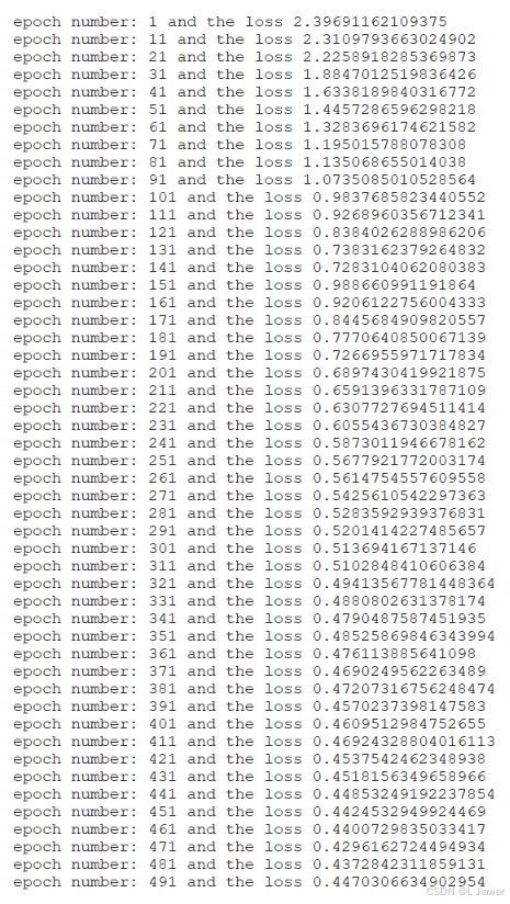
在第420轮左右误差有小幅增大,但测试结果良好:

测试准确率由 80.33% 增至 90.18%。
将总训练轮数调至400轮,训练准确率更高。
这虽然 简单说明 了 深度网络优于浅层网络,但因原始数据集不能代表所有未知数据,且该数据集同质化数据较高,未考虑 背景色 等因素,故仍不能排除存在 过拟合 的可能性,结果仍存在疑点。
但毫无疑问的是,深层网络具有更多权重,容量大。且网络结构“更深”,可以逐步过滤提取特征,提取深层隐藏特征,最终输出更优的结果。
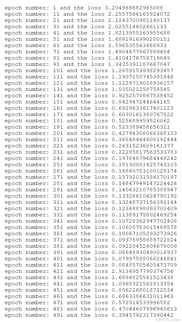
训练过程:
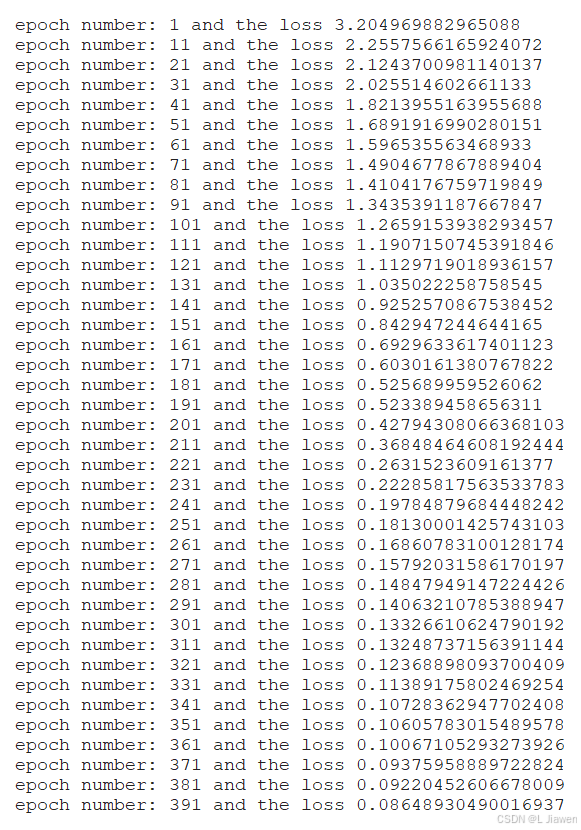
测试结果:

测试准确率由 90.18% 增至 94.95%。
其实,从两个图像识别分类任务比对也可看出,衣物图标任务数据集表现形式更丰富,若想达到与手写数字任务 相近/更优 的准确率,需使用 更深+更复杂 的神经网络。
②【衣物图标】Dropout 提升精准度
引入Dropout,该识别分类实验准确率得以破8。
去除该实验中所有层Dropout,从第100轮左右可看出神经网络收敛速度相较于引入Dropout更快,但最终结果较差:
训练过程:
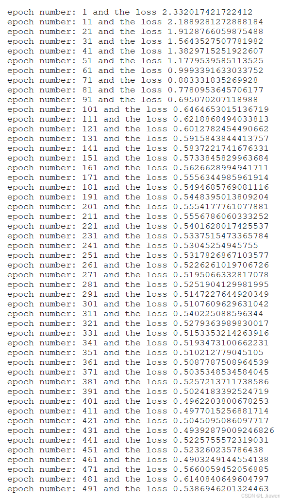
测试结果:

测试准确率由 80.33% 降至 78.05%。
9.2.4 保存&加载 模型
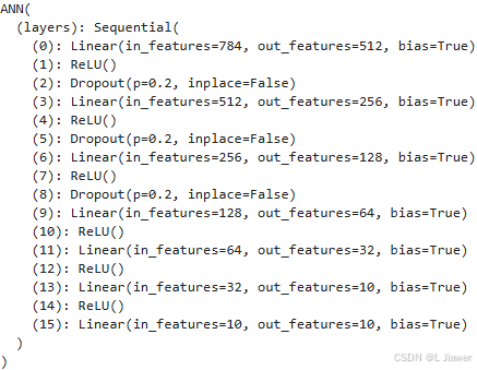
以附带Dropout的衣物图标识别为例:
保存模型
torch.save(model.state_dict(),'fashion-mnist-ANN.pt')
加载模型
model = MyANN()

model.load_state_dict(torch.load('fashion-mnist-ANN.pt'))
print(model)		# 可查看网络结构
9.3 预测回归
(1) 数据集介绍
California房价预测数据集
California房价预测数据集,为Boston房价数据集的平替数据集。
fetch系列数据集需要通过网络下载,但有时会抛出HTTPError: HTTP Error 403: Forbidden的异常。
# Scikit-learn
# california 房价预测数据集
from sklearn.datasets import fetch_california_housing
from sklearn.model_selection import train_test_split

housing_california = fetch_california_housing()
X = housing_california.data    # data
y = housing_california.target   # label
故可以通过网址自行 下载,再通过tarfile库读取数据。
下载地址:https://www.dcc.fc.up.pt/~ltorgo/Regression/cal_housing.tgz
import pandas as pd
import tarfile
from sklearn.model_selection import train_test_split

tar = tarfile.open(r'./data/cal_housing.tgz')
names = tar.getnames()         # ['CaliforniaHousing/cal_housing.data', 'CaliforniaHousing/cal_housing.domain']

# 抽取.data文件,其格式等同csv文件
data = tar.extractfile(names[0])
df = pd.read_csv(data, header=None)
# 抽取.domain文件,其格式等同csv文件
domain = tar.extractfile(names[1])
ddf = pd.read_csv(domain, header=None)
ddf = ddf.values.tolist()
headers = []
for ddff in ddf:
    header = ddff[0].split(':')[0]
    headers.append(header)

# 更换表头,更加直观;亦可不换,直转Tensor。
df.columns = headers
(2) 训练模型
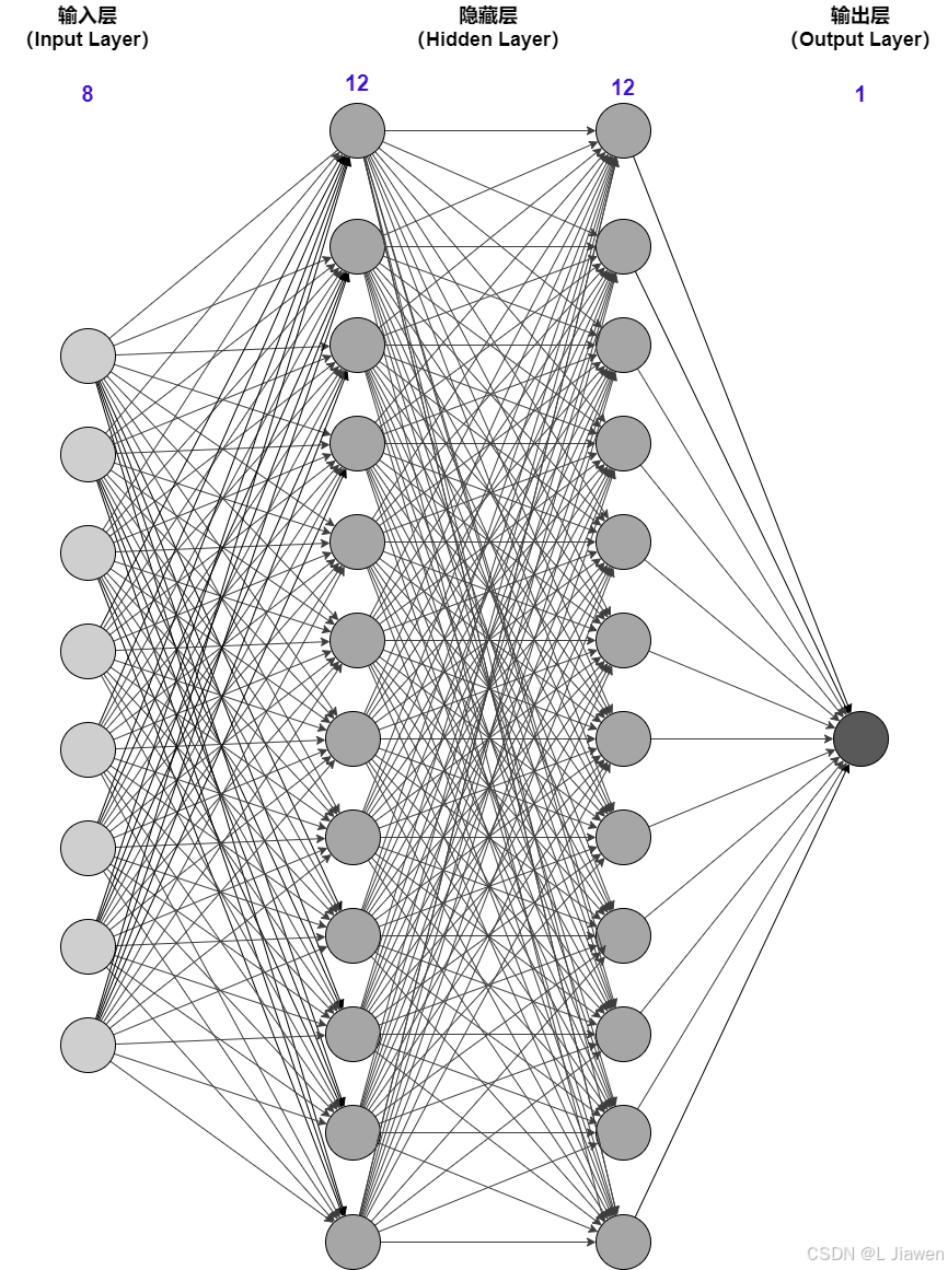
绘制网络结构图
① 导入三方库
import torch
import torch.nn as nn
import numpy as np
② 读取数据集
sklearn.model_selection读取
# Scikit-learn
# california 房价预测数据集
from sklearn.datasets import fetch_california_housing
from sklearn.model_selection import train_test_split

housing_california = fetch_california_housing()
X = housing_california.data    # data
y = housing_california.target   # label
文件读取
import pandas as pd
import tarfile
from sklearn.model_selection import train_test_split

tar = tarfile.open(r'./data/cal_housing.tgz')
names = tar.getnames()         # ['CaliforniaHousing/cal_housing.data', 'CaliforniaHousing/cal_housing.domain']

# 抽取.data文件,其格式等同csv文件
data = tar.extractfile(names[0])
df = pd.read_csv(data, header=None)
# 抽取.domain文件,其格式等同csv文件
domain = tar.extractfile(names[1])
ddf = pd.read_csv(domain, header=None)
ddf = ddf.values.tolist()
headers = []
for ddff in ddf:
    header = ddff[0].split(':')[0]
    headers.append(header)

# 更换表头,更加直观;亦可不换,直转Tensor。
df.columns = headers
读取数据
data = df.values

from sklearn.preprocessing import MinMaxScaler
scaler = MinMaxScaler()
scaler = scaler.fit(data)

result = scaler.transform(data)
print(result)

X = result[:,:-1]
y = result[:,-1:]
划分数据集
X_train, X_test, y_train, y_test = train_test_split(X, y, random_state=12, test_size=0.2)
X_train = torch.Tensor(X_train)
X_test = torch.Tensor(X_test)
y_train = torch.Tensor(y_train)
y_test = torch.Tensor(y_test)
③ 创建人工神经网络
class ANN(nn.Module):
    n_input = 8
    n_h1 = 12
    n_h2 = 12
    n_output = 1

    def __init__(self):
        super(ANN, self).__init__()

        self.layers = nn.Sequential (
            nn.Linear(self.n_input, self.n_h1),
            nn.ReLU(),
            nn.Linear(self.n_h1, self.n_h2),
            nn.ReLU(),
            nn.Linear(self.n_h2, self.n_output),
        )

    def forward(self, x):
        return self.layers(x)
④ 训练人工神经网络
# 设置随机种子,确保结果一致
# torch.manual_seed(24)
# 创建模型对象
model = ANN()

# 定义损失函数
loss_function = nn.MSELoss()
# 定义优化器
optimizer = torch.optim.Adam(model.parameters(), lr=0.01)

# 定义轮次
epochs = 500
batch_size = 50
# 累计损失
final_losses = []

for i in range(epochs):
    count = 0
    for j in range(batch_size):
        # 1. 正向传播
        y_pred = model(X_train[count*batch_size:count*batch_size+batch_size])
        # 2. 计算损失
        loss = loss_function(y_pred, y_train[count*batch_size:count*batch_size+batch_size])
        final_losses.append(loss)

        # 清空梯度
        optimizer.zero_grad()
        # 3. 反向传播
        loss.backward()
        # 4. 优化参数
        optimizer.step()
        count+=1

    if i % 10 == 0:
        print("epoch number: {} and the loss {}".format(i+1, loss.item()))
⑤ 测试人工神经网络
total = len(X_test)
currect = 0

with torch.no_grad():
    for i in range(total):
        outputs = model(X_test[i])
        if abs(outputs - y_test[i]) - 0.1 < 0:
            currect+=1
print('Test Currect Rate: {}%'.format(currect / total * 100))


 9万+
9万+

 被折叠的 条评论
为什么被折叠?
被折叠的 条评论
为什么被折叠?
 到【灌水乐园】发言


