


- 🍨 本文为🔗365天深度学习训练营 中的学习记录博客
- 🍖 原作者:K同学啊
一、前期准备
1.设置GPU
import torch
import torch.nn as nn
import torchvision.transforms as transforms
import torchvision
from torchvision import transforms,datasets
import os,PIL,pathlib,random

device = torch.device("cuda" if torch.cuda.is_available() else "cpu")
device
device(type=‘cuda’)
2.导入数据
data_dir = r"D:\z_temp\data\weather_photos"
data_dir = pathlib.Path(data_dir)

data_paths = list(data_dir.glob('*'))
classeNames = [str(path).split("\\")[4] for path in data_paths]
classeNames
[‘cloudy’, ‘rain’, ‘shine’, ‘sunrise’]
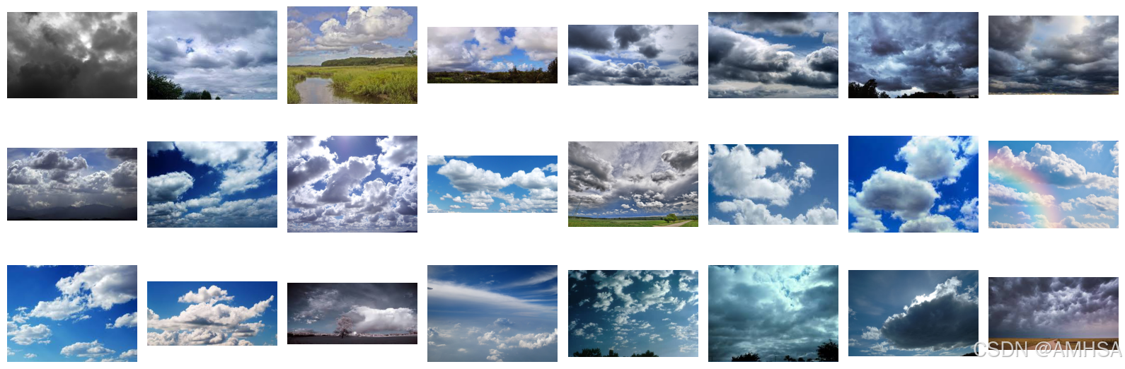
3.查看数据
import matplotlib.pyplot as plt
from PIL import Image

image_folder = r'D:\z_temp\data\weather_photos\cloudy'
image_files = [f for f in os.listdir(image_folder) if f.endswith((".jpg",".png",".jepg"))]

fig,axex = plt.subplots(3,8,figsize=(16,6))

for ax,img_file in zip(axex.flat,image_files):#将axex3*8的二维数组拉成一维24
    img_path = os.path.join(image_folder,img_file)
    img = Image.open(img_path)
    ax.imshow(img)
    ax.axis('off')

plt.tight_layout()
plt.show()
total_datadir = r"D:\z_temp\data\weather_photos"
train_transforms = transforms.Compose([
    transforms.Resize([224,224]),
    transforms.ToTensor(),
    transforms.Normalize(           #对每个通道(RGB)进行 标准化
        mean=[0.485,0.456,0.406],
        std=[0.229,0.224,0.225])
])
#mean/std 取自 ImageNet,是因为很多预训练模型(ResNet、VGG)是基于 ImageNet 训练的,
#使用相同的均值和标准差可以 让数据分布更匹配模型期望的输入。

total_data = datasets.ImageFolder(total_datadir,transform = train_transforms)
total_data
Dataset ImageFolder
Number of datapoints: 1125
Root location: D:\z_temp\data\weather_photos
StandardTransform
Transform: Compose(
Resize(size=[224, 224], interpolation=bilinear, max_size=None, antialias=True)
ToTensor()
Normalize(mean=[0.485, 0.456, 0.406], std=[0.229, 0.224, 0.225])
)
4.划分数据集
train_size = int(0.8*len(total_data))
test_size  = len(total_data)-train_size
train_dataset,test_dataset = torch.utils.data.random_split(total_data,[train_size,test_size])
train_dataset,test_dataset
(<torch.utils.data.dataset.Subset at 0x21e950153d0>,
<torch.utils.data.dataset.Subset at 0x21e95015460>)
batch_size = 32
train_dl = torch.utils.data.DataLoader(train_dataset,
                                      batch_size = batch_size,
                                      shuffle = True,
                                      num_workers = 1)
test_dl = torch.utils.data.DataLoader(test_dataset,
                                      batch_size = batch_size,
                                      shuffle = True,
                                      num_workers = 1)

for X, y in test_dl:
    print("Shape of X [N, C, H, W]: ", X.shape)
    print("Shape of y: ", y.shape, y.dtype)
    break
Shape of X [N, C, H, W]: torch.Size([32, 3, 224, 224])
Shape of y: torch.Size([32]) torch.int64
二、构建CNN
import torch.nn.functional as F

class Network_bn(nn.Module):
    def __init__(self):
        super(Network_bn,self).__init__()
        self.conv1 = nn.Conv2d(in_channels = 3,
                              out_channels = 12,
                              kernel_size = 5,
                              stride = 1,
                              padding = 0)
        #在卷积神经网络(CNN)中应用批量归一化(Batch Normalization,简称 BN)的操作
        #它的作用是在训练时对每个批次(batch)的数据进行标准化, 加速训练,提高模型稳定性,减少过拟合。
        self.bn1 = nn.BatchNorm2d(12)
        self.conv2 = nn.Conv2d(in_channels = 12,
                              out_channels = 12,
                              kernel_size = 5,
                              stride = 1,
                              padding = 0)
        self.bn2 = nn.BatchNorm2d(12)
        self.pool1 = nn.MaxPool2d(2,2)
        self.conv4 = nn.Conv2d(in_channels = 12,
                              out_channels = 24,
                              kernel_size = 5,
                              stride = 1,
                              padding = 0)
        self.bn4 = nn.BatchNorm2d(24)
        self.conv5 = nn.Conv2d(in_channels = 24,
                              out_channels = 24,
                              kernel_size = 5,
                              stride = 1,
                              padding = 0)
        self.bn5 = nn.BatchNorm2d(24)
        self.pool2 = nn.MaxPool2d(2,2)
        #遗留问题:为什么两个卷积+一个池化?
        #cnn的结构怎那么设计?
        self.fc1 = nn.Linear(24*50*50,len(classeNames))

    def forward(self,x):
        x = F.relu(self.bn1(self.conv1(x)))
        x = F.relu(self.bn2(self.conv2(x)))
        x = self.pool1(x)
        x = F.relu(self.bn4(self.conv4(x)))
        x = F.relu(self.bn5(self.conv5(x)))
        x = self.pool2(x)
        x = x.view(-1,24*50*50)#相当于flatten
        x = self.fc1(x)

        return x

device = "cuda" if torch.cuda.is_available() else "cpu"
print("Using {} device".format(device))

model = Network_bn().to(device)
model
Network_bn(
(conv1): Conv2d(3, 12, kernel_size=(5, 5), stride=(1, 1))
(bn1): BatchNorm2d(12, eps=1e-05, momentum=0.1, affine=True, track_running_stats=True)
(conv2): Conv2d(12, 12, kernel_size=(5, 5), stride=(1, 1))
(bn2): BatchNorm2d(12, eps=1e-05, momentum=0.1, affine=True, track_running_stats=True)
(pool1): MaxPool2d(kernel_size=2, stride=2, padding=0, dilation=1, ceil_mode=False)
(conv4): Conv2d(12, 24, kernel_size=(5, 5), stride=(1, 1))
(bn4): BatchNorm2d(24, eps=1e-05, momentum=0.1, affine=True, track_running_stats=True)
(conv5): Conv2d(24, 24, kernel_size=(5, 5), stride=(1, 1))
(bn5): BatchNorm2d(24, eps=1e-05, momentum=0.1, affine=True, track_running_stats=True)
(pool2): MaxPool2d(kernel_size=2, stride=2, padding=0, dilation=1, ceil_mode=False)
(fc1): Linear(in_features=60000, out_features=4, bias=True)
)
三、训练模型
1.设置超参数
loss_fn = nn.CrossEntropyLoss()
learn_rate = 1e-4
opt = torch.optim.SGD(model.parameters(),lr=learn_rate)
2.编写训练函数
def train(dataloader,model,loss_fn,optimizer):
    size = len(dataloader.dataset)
    num_batches = len(dataloader)

    train_loss,train_acc = 0,0

    for X,y in dataloader:
        X,y = X.to(device),y.to(device)

        pred = model(X)
        loss = loss_fn(pred,y)

        optimizer.zero_grad()
        loss.backward()
        optimizer.step()

        train_acc += (pred.argmax(1) == y).type(torch.float).sum().item()
        train_loss += loss.item()

    train_acc /= size
    train_loss /= num_batches

    return train_acc,train_loss
3.编写测试函数
def test(dataloader,model,loss_fn):
    size = len(dataloader.dataset)
    num_batches = len(dataloader)
    test_loss,test_acc = 0,0

    with torch.no_grad():
        for imgs,target in dataloader:
            imgs,target = imgs.to(device),target.to(device)

            target_pred = model(imgs)
            loss = loss_fn(target_pred,target)

            test_loss += loss.item()
            test_acc += (target_pred.argmax(1) == target).type(torch.float).sum().item()

    test_acc /= size
    test_loss /= num_batches

    return test_acc, test_loss
4.正式训练
epochs     = 20
train_loss = []
train_acc  = []
test_loss  = []
test_acc   = []

for epoch in range(epochs):
    model.train()
    epoch_train_acc, epoch_train_loss = train(train_dl, model, loss_fn, opt)

    model.eval()
    epoch_test_acc, epoch_test_loss = test(test_dl, model, loss_fn)

    train_acc.append(epoch_train_acc)
    train_loss.append(epoch_train_loss)
    test_acc.append(epoch_test_acc)
    test_loss.append(epoch_test_loss)

    template = ('Epoch:{:2d}, Train_acc:{:.1f}%, Train_loss:{:.3f}, Test_acc:{:.1f}%,Test_loss:{:.3f}')
    print(template.format(epoch+1, epoch_train_acc*100, epoch_train_loss, epoch_test_acc*100, epoch_test_loss))
print('Done')
Epoch: 1, Train_acc:77.0%, Train_loss:0.637, Test_acc:72.0%,Test_loss:0.769
Epoch: 2, Train_acc:80.0%, Train_loss:0.544, Test_acc:81.3%,Test_loss:0.506
Epoch: 3, Train_acc:84.6%, Train_loss:0.493, Test_acc:75.1%,Test_loss:0.540
Epoch: 4, Train_acc:86.0%, Train_loss:0.415, Test_acc:81.3%,Test_loss:0.546
Epoch: 5, Train_acc:86.6%, Train_loss:0.388, Test_acc:82.7%,Test_loss:0.477
Epoch: 6, Train_acc:88.1%, Train_loss:0.370, Test_acc:84.0%,Test_loss:0.423
Epoch: 7, Train_acc:90.4%, Train_loss:0.323, Test_acc:85.3%,Test_loss:0.401
Epoch: 8, Train_acc:89.8%, Train_loss:0.359, Test_acc:88.0%,Test_loss:0.354
Epoch: 9, Train_acc:91.1%, Train_loss:0.322, Test_acc:82.2%,Test_loss:0.433
Epoch:10, Train_acc:91.0%, Train_loss:0.343, Test_acc:80.0%,Test_loss:0.456
Epoch:11, Train_acc:92.3%, Train_loss:0.270, Test_acc:87.1%,Test_loss:0.344
Epoch:12, Train_acc:93.6%, Train_loss:0.247, Test_acc:88.9%,Test_loss:0.337
Epoch:13, Train_acc:93.8%, Train_loss:0.246, Test_acc:88.9%,Test_loss:0.310
Epoch:14, Train_acc:93.0%, Train_loss:0.270, Test_acc:88.9%,Test_loss:0.350
Epoch:15, Train_acc:94.3%, Train_loss:0.215, Test_acc:89.3%,Test_loss:0.308
Epoch:16, Train_acc:95.0%, Train_loss:0.194, Test_acc:88.4%,Test_loss:0.319
Epoch:17, Train_acc:95.8%, Train_loss:0.196, Test_acc:89.8%,Test_loss:0.282
Epoch:18, Train_acc:95.0%, Train_loss:0.199, Test_acc:88.0%,Test_loss:0.315
Epoch:19, Train_acc:95.0%, Train_loss:0.195, Test_acc:89.8%,Test_loss:0.343
Epoch:20, Train_acc:95.4%, Train_loss:0.205, Test_acc:90.7%,Test_loss:0.299
Done
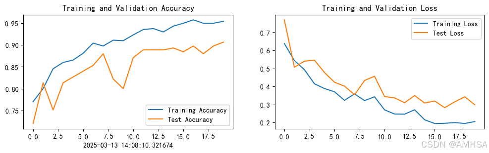
四、结果可视化
import matplotlib.pyplot as plt
#隐藏警告
import warnings
warnings.filterwarnings("ignore")               #忽略警告信息
plt.rcParams['font.sans-serif']    = ['SimHei'] # 用来正常显示中文标签
plt.rcParams['axes.unicode_minus'] = False      # 用来正常显示负号
plt.rcParams['figure.dpi']         = 100        #分辨率

from datetime import datetime
current_time = datetime.now() # 获取当前时间

epochs_range = range(epochs)

plt.figure(figsize=(12, 3))
plt.subplot(1, 2, 1)

plt.plot(epochs_range, train_acc, label='Training Accuracy')
plt.plot(epochs_range, test_acc, label='Test Accuracy')
plt.legend(loc='lower right')
plt.title('Training and Validation Accuracy')
plt.xlabel(current_time) # 打卡请带上时间戳,否则代码截图无效

plt.subplot(1, 2, 2)
plt.plot(epochs_range, train_loss, label='Training Loss')
plt.plot(epochs_range, test_loss, label='Test Loss')
plt.legend(loc='upper right')
plt.title('Training and Validation Loss')
plt.show()
五、调用模型测试
torch.save(model.state_dict(), "model.pth")  # 训练时运行这行代码保存模型
import torch
from PIL import Image
import torchvision.transforms as transforms

# 1. 设备检测
device = torch.device("cuda" if torch.cuda.is_available() else "cpu")

# 2. 加载模型
model = Network_bn().to(device)  # 确保你有 Network_bn 这个类
model.load_state_dict(torch.load("model.pth", map_location=device))
model.eval()

# 3. 定义数据预处理
transform = transforms.Compose([
    transforms.Resize((224, 224)),
    transforms.ToTensor(),
    transforms.Normalize(mean=[0.485, 0.456, 0.406], std=[0.229, 0.224, 0.225])
])

# 4. 读取并预处理本地图片
image_path = r"C:\Users\as\Desktop\004940d89e4ee485e5ad3c02b18065e.jpg"
image = Image.open(image_path)
image = transform(image).unsqueeze(0).to(device)

# 5. 进行预测
with torch.no_grad():
    output = model(image)
    prediction = torch.argmax(output, dim=1)

# 6. 显示预测类别
print(f"Predicted class: {classeNames[prediction.item()]}")
Predicted class: sunrise
我的图片:


 被折叠的 条评论
为什么被折叠?
被折叠的 条评论
为什么被折叠?
 到【灌水乐园】发言


