


6.1 图像噪声加入
给图像加入高斯噪声和椒盐噪声,需要我们了解以下代码:
①img_g = skimage.util.random_noise(img, 'gaussian', mean=0, var=0.05):
这行代码的作用是给图像img添加高斯噪声。
'gaussian':表示要添加的噪声类型为高斯噪声。高斯噪声是一种符合高斯分布的随机噪声。
mean=0:表示高斯噪声的均值为 0。这意味着噪声的平均值是 0,噪声值会在 0 附近波动。
var=0.05:表示高斯噪声的方差为 0.05。方差反映了噪声的分散程度,方差越大,噪声的波动范围就越大。
②img_s = skimage.util.random_noise(img, 'salt'):
这行代码是给图像img添加椒盐噪声中的盐噪声。
'salt':代表要添加的噪声类型为盐噪声。盐噪声会随机地将图像中的一些像素值设为最大值,看起来就像图像上有白色的 “盐粒”。
代码如下及运行结果如图3.21。
import skimage
import cv2
import matplotlib.pylab as plt
plt.rcParams['font.sans-serif'] = ['SimHei']
plt.rcParams['axes.unicode_minus'] = False
img = cv2.imread('002.bmp', 0)
img = img / 255
img_g = skimage.util.random_noise(img, 'gaussian', mean=0, var=0.05)
img_s = skimage.util.random_noise(img, 'salt')
plt.subplot(131)
plt.imshow(img, 'gray')
plt.title('原图')
plt.subplot(132)
plt.imshow(img_g, 'gray')
plt.title('加入高斯噪声后图像')
plt.subplot(133)
plt.imshow(img_s, 'gray')
plt.title('加入椒盐噪声后图像')
plt.show()
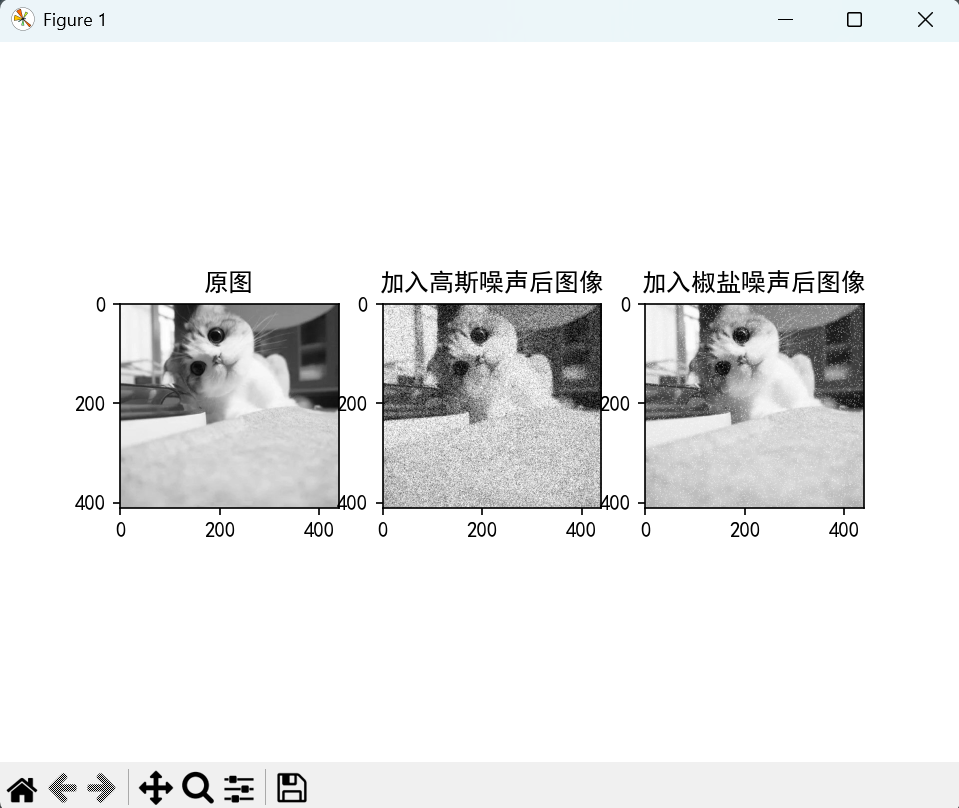
通过上述代码,我们给图像加入了高斯噪声和椒盐噪声。
6.2 图像空域滤波
6.2.1 空域平滑滤波
邻均值滤波是最简单的空域平滑滤波方法,在使用邻均值滤波前我们需了解以下代码:
cv2.blur(img_g, (3, 3)):
img_g:这是一张添加噪声后的图像。
(3, 3):这是滤波核的大小,也称为卷积核或窗口大小。它是一个二元组,这里表示一个 3x3 的矩阵。在进行均值滤波时,会在图像上滑动这个 3x3 的窗口,计算窗口内所有像素的平均值,并将该平均值作为窗口中心像素的新值。
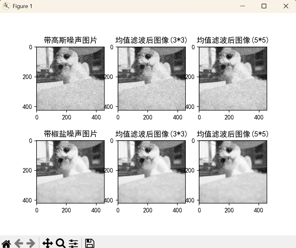
代码如下及运行结果如图3.22。
import cv2
import matplotlib.pyplot as plt
plt.rcParams['font.sans-serif'] = ['SimHei']
plt.rcParams['axes.unicode_minus'] = False
img_g = cv2.imread('002_g.bmp', 0)
img_s = cv2.imread('002_s.bmp', 0)
img_g_l = cv2.blur(img_g, (3, 3))
img_s_l = cv2.blur(img_s, (3, 3))
img_g_l1 = cv2.blur(img_g, (5, 5))
img_s_l1 = cv2.blur(img_s, (5, 5))
plt.subplot(231)
plt.imshow(img_g, 'gray')
plt.title('带高斯噪声图片')
plt.subplot(234)
plt.imshow(img_s, 'gray')
plt.title('带椒盐噪声图片')
plt.subplot(232)
plt.imshow(img_g_l, 'gray')
plt.title('均值滤波后图像(3*3)')
plt.subplot(233)
plt.imshow(img_g_l1, 'gray')
plt.title('均值滤波后图像(5*5)')
plt.subplot(235)
plt.imshow(img_s_l, 'gray')
plt.title('均值滤波后图像(3*3)')
plt.subplot(236)
plt.imshow(img_s_l1, 'gray')
plt.title('均值滤波后图像(5*5)')
plt.show()
根据结果可以看到两种噪声在均值滤波后都一定程度上减少了,但是图片也变得模糊。随着滤波器变大,去噪效果变好,但是模糊程度变更大。为了能够获取更好的滤波效果同时又保证图像的清晰度,我们可以使用加权平均滤波器,如高斯滤波器。我们需了解以下代码:
img_g_l = cv2.GaussianBlur(img_g, (3, 3), 0, 5):
这行代码的作用是对输入图像img_g进行高斯滤波。
(3, 3):表示高斯核的大小,是一个二元组。这里 (3, 3) 代表一个 3x3 的高斯核,在进行高斯滤波时,会以每个像素为中心,考虑其周围 3x3 邻域内的像素值。
0:表示X方向上的高斯核标准差。如果将其设置为 0,OpenCV 会根据高斯核的大小自动计算合适的标准差。
代码如下及运行结果如图3.23。
import cv2
import matplotlib.pyplot as plt
plt.rcParams['font.sans-serif'] = ['SimHei']
plt.rcParams['axes.unicode_minus'] = False
img_g = cv2.imread('002_g.bmp', 0)
img_s = cv2.imread('002_s.bmp', 0)
img_g_l = cv2.GaussianBlur(img_g, (3, 3), 0, 5)
img_s_l = cv2.GaussianBlur(img_s, (3, 3), 0, 5)
img_g_l1 = cv2.GaussianBlur(img_g, (5, 5), 0, 5)
img_s_l1 = cv2.GaussianBlur(img_s, (5, 5), 0, 5)
plt.subplot(231)
plt.imshow(img_g, 'gray')
plt.title('带高斯噪声图片')
plt.subplot(234)
plt.imshow(img_s, 'gray')
plt.title('带椒盐噪声图片')
plt.subplot(232)
plt.imshow(img_g_l, 'gray')
plt.title('高斯滤波后图像(3*3)')
plt.subplot(233)
plt.imshow(img_g_l1, 'gray')
plt.title('高斯滤波后图像(5*5)')
plt.subplot(235)
plt.imshow(img_s_l, 'gray')
plt.title('高斯滤波后图像(3*3)')
plt.subplot(236)
plt.imshow(img_s_l1, 'gray')
plt.title('高斯滤波后图像(5*5)')
plt.show()
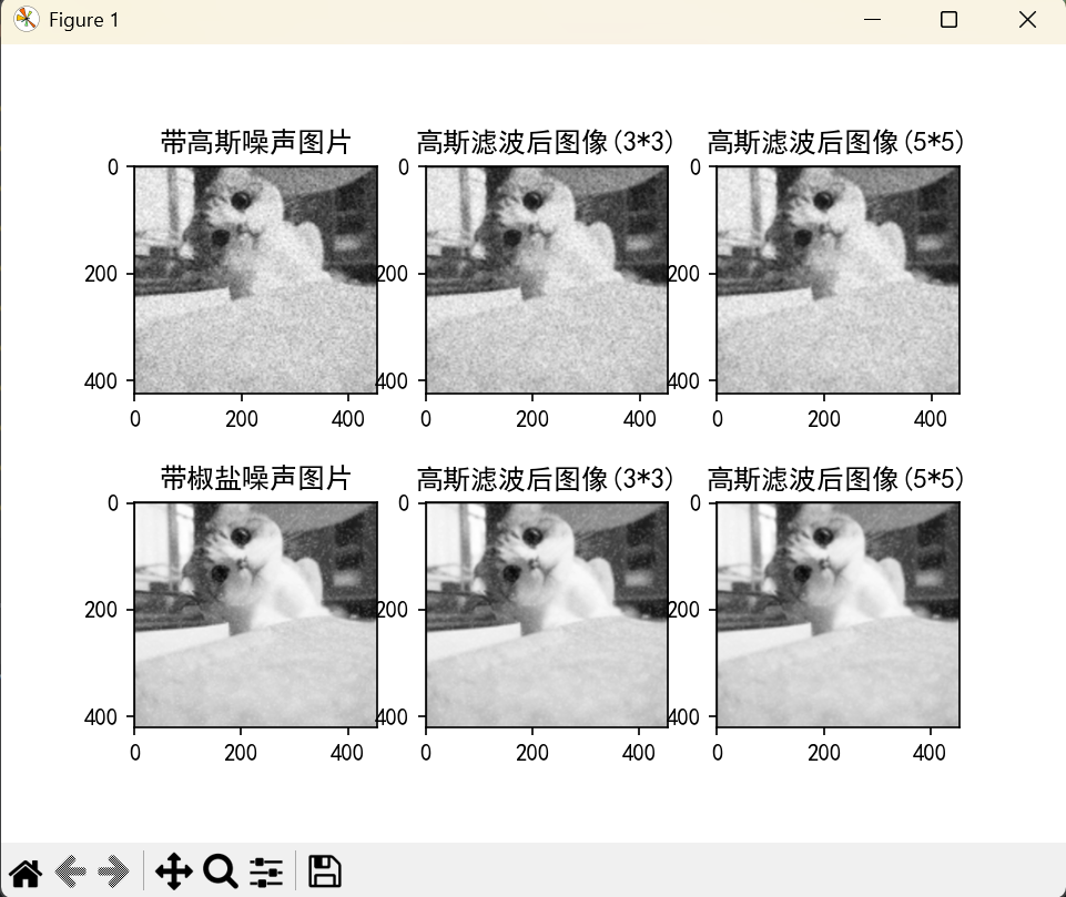
根据结果可以看到高斯滤波和均值滤波类似,但高斯滤波后图像清晰度要比均值滤波的高。常用的空域滤波还有非线性的中值滤波器。同样,我们需了解以下代码:
img_g_l = cv2.medianBlur(img_g, 3):
3:表示滤波核的大小,这里是 3。滤波核的大小必须是大于 1 的奇数。在进行中值滤波时,会在图像上滑动一个边长为 3 的正方形窗口,将窗口内所有像素值排序后取中间值作为窗口中心像素的新值。
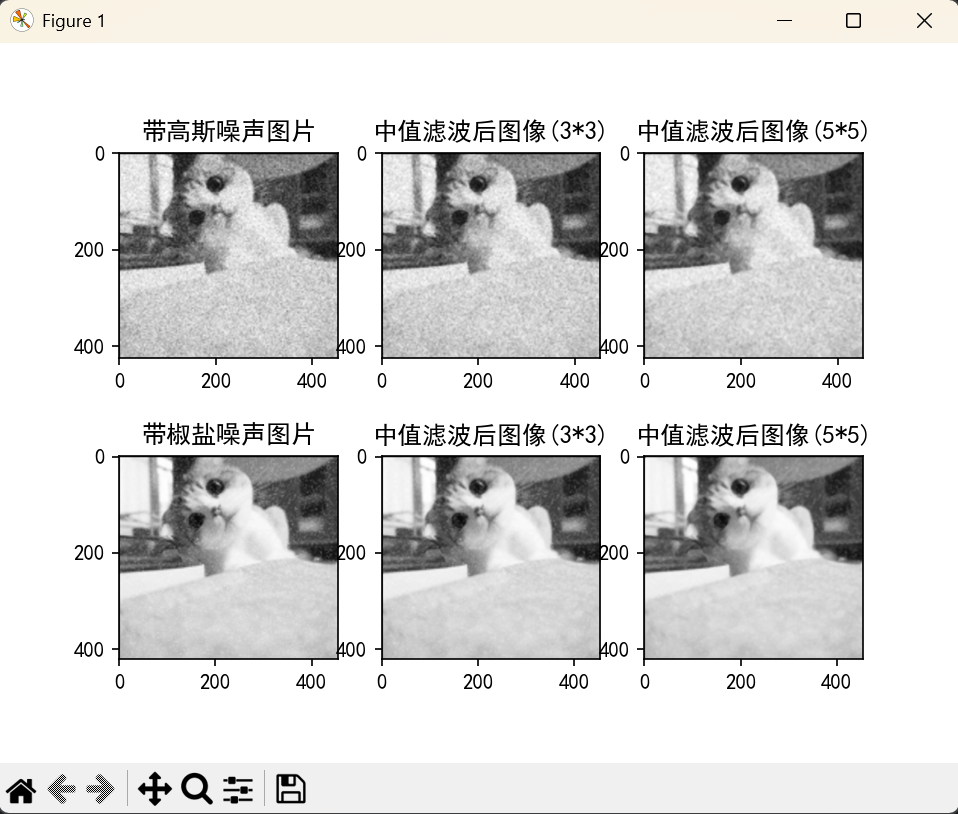
代码如下及运行结果如图3.24。
import cv2
import matplotlib.pyplot as plt
plt.rcParams['font.sans-serif'] = ['SimHei']
plt.rcParams['axes.unicode_minus'] = False
img_g = cv2.imread('002_g.bmp', 0)
img_s = cv2.imread('002_s.bmp', 0)
img_g_l = cv2.medianBlur(img_g, 3)
img_s_l = cv2.medianBlur(img_s, 3)
img_g_l1 = cv2.medianBlur(img_g, 5)
img_s_l1 = cv2.medianBlur(img_s, 5)
plt.subplot(231)
plt.imshow(img_g, 'gray')
plt.title('带高斯噪声图片')
plt.subplot(234)
plt.imshow(img_s, 'gray')
plt.title('带椒盐噪声图片')
plt.subplot(232)
plt.imshow(img_g_l, 'gray')
plt.title('中值滤波后图像(3*3)')
plt.subplot(233)
plt.imshow(img_g_l1, 'gray')
plt.title('中值滤波后图像(5*5)')
plt.subplot(235)
plt.imshow(img_s_l, 'gray')
plt.title('中值滤波后图像(3*3)')
plt.subplot(236)
plt.imshow(img_s_l1, 'gray')
plt.title('中值滤波后图像(5*5)')
plt.show()
根据结果可得中值滤波对椒盐噪声有更好的滤波效果。
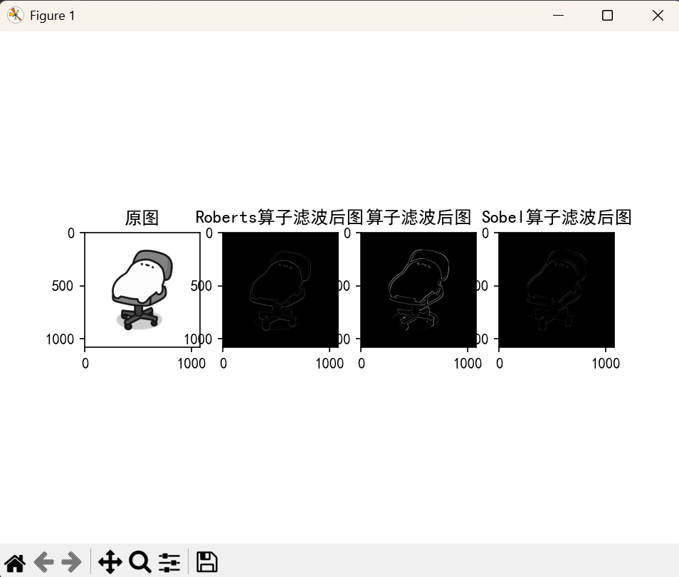
6.2.2 空域锐化滤波
空域锐化常用的方式是通过梯度算子进行滤波,一般使用的梯度算子有Roberts、Prewitt和Sobel等。我们需了解以下代码:
①Roberts算子:
罗伯特算子是一种简单的边缘检测算子,通过计算图像中像素的梯度来检测边缘。
Robertx = np.array([[-1, 0], [0, 1]]) Roberty = np.array([[0, -1], [1, 0]])
这两行代码分别定义了罗伯特算子在水平方向和垂直方向上的卷积核。Robertx 卷积核用于检测水平方向的边缘变化,Roberty 卷积核用于检测垂直方向的边缘变化。
img_x = cv2.filter2D(img, -1, Robertx) img_y = cv2.filter2D(img, -1, Roberty)
这两行代码使用 cv2.filter2D函数对输入图像img分别进行二维卷积操作。
-1:表示输出图像的数据类型与输入图像相同。
②Sobel算子:
img_s = cv2.Sobel(img, -1, 1, 1)
1:第一个 1 表示在 x 方向上求导的阶数。设置为1意味着要计算图像在 x 方向上的一阶导数,即检测图像在水平方向上的边缘变化。
1:第二个 1 表示在 y 方向上求导的阶数。设置为1意味着要计算图像在 y 方向上的一阶导数,即检测图像在垂直方向上的边缘变化。
代码如下及运行结果如图3.25。
import cv2
import matplotlib.pyplot as plt
import numpy as np
plt.rcParams['font.sans-serif'] = ['SimHei']
plt.rcParams['axes.unicode_minus'] = False
img = cv2.imread('001.bmp', 0)
# Roberts
Robertx = np.array([[-1, 0], [0, 1]])
Roberty = np.array([[0, -1], [1, 0]])
img_x = cv2.filter2D(img, -1, Robertx)
img_y = cv2.filter2D(img, -1, Roberty)
img_r = abs(img_x) + abs(img_y)
# Prewitt
Prewittx = np.array([[1, 1, 1], [0, 0, 0], [-1, -1, -1]])
Prewitty = np.array([[-1, 0, 1], [-1, 0, 1], [-1, 0, 1]])
img_x = cv2.filter2D(img, -1, Prewittx)
img_y = cv2.filter2D(img, -1, Prewitty)
img_p = abs(img_x) + abs(img_y)
# Sobel
img_s = cv2.Sobel(img, -1, 1, 1)
plt.subplot(141)
plt.imshow(img, 'gray')
plt.title('原图')
plt.subplot(142)
plt.imshow(img_r, 'gray')
plt.title('Roberts算子滤波后图')
plt.subplot(143)
plt.imshow(img_p, 'gray')
plt.title('Prewitt算子滤波后图')
plt.title('算子滤波后图')
plt.subplot(144)
plt.imshow(img_s, 'gray')
plt.title('Sobel算子滤波后图')
plt.show()
6.3 拓展
6.3.1 拓展1
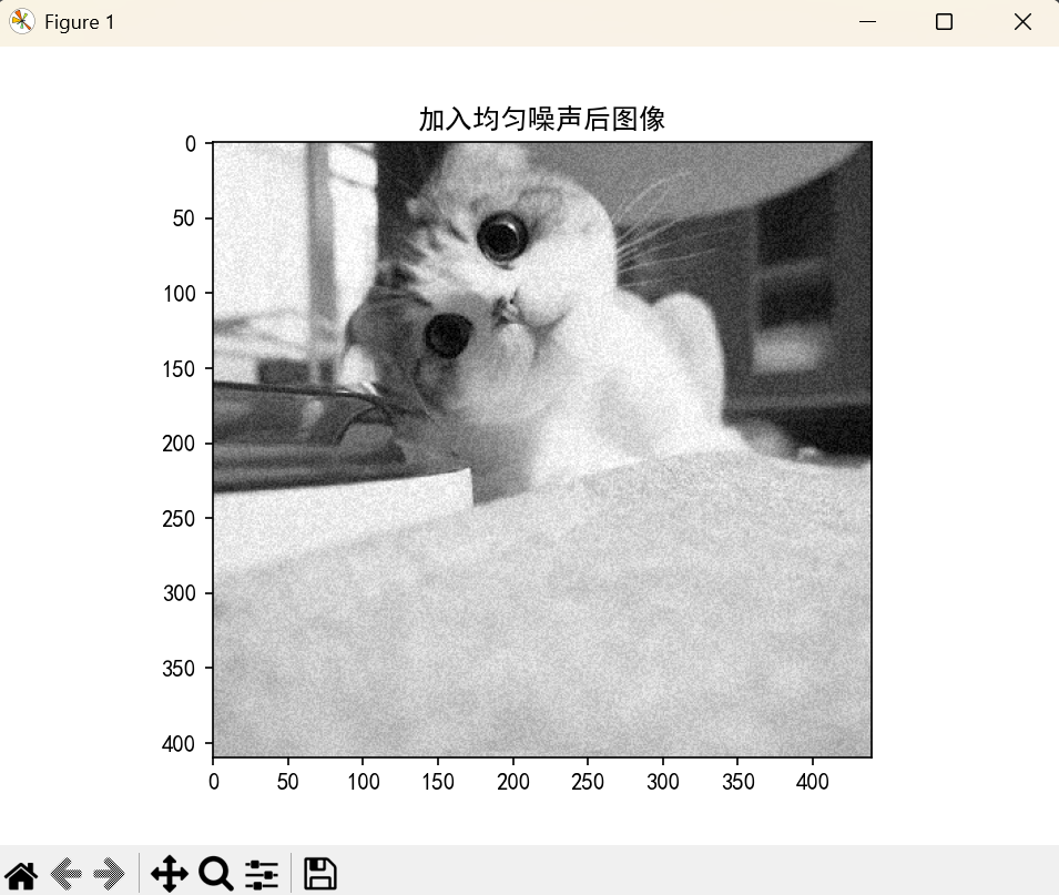
题目:写一个程序,分别对一幅被均匀噪声和椒盐噪声污染的图像,用均值滤波、高斯滤波和中值滤波器处理,对比分析结果。
要想完成拓展题目,首先我们需要生成一幅带有均匀噪声的图像,代码如下及运行结果如图3.21.jyzs。
import cv2
import numpy as np
import matplotlib.pylab as plt
plt.rcParams['font.sans-serif'] = ['SimHei']
plt.rcParams['axes.unicode_minus'] = False
img = cv2.imread('002.bmp', 0)
img = img.astype(float)  # 将图像像素值转换为浮点型,方便后续计算
rows, cols = img.shape  # 获取图像的行数和列数
# 生成均匀分布的随机噪声,范围在[-a, a],这里a设为20
noise = np.random.uniform(-20, 20, (rows, cols))
img_u = img + noise
# 对像素值进行截断,确保在0 - 255范围内
img_u = np.clip(img_u, 0, 255)
# 转换回uint8类型
img_u = img_u.astype(np.uint8)
plt.imshow(img_u, 'gray')
plt.title('加入均匀噪声后图像')
plt.show()
然后,根据前文所学内容,即可完成拓展题目,代码如下及运行结果如图tz1。
import cv2
import matplotlib.pylab as plt
plt.rcParams['font.sans-serif'] = ['SimHei']
plt.rcParams['axes.unicode_minus'] = False
img_u = cv2.imread('002_u.bmp', 0)
img_s = cv2.imread('002_s.bmp', 0)
#  均值滤波
img_u_l = cv2.blur(img_u, (5, 5))
img_s_l = cv2.blur(img_s, (5, 5))
#  高斯滤波
img_u_l1 = cv2.GaussianBlur(img_u, (5, 5), 0, 5)
img_s_l1 = cv2.GaussianBlur(img_s, (5, 5), 0, 5)
#  中值滤波
img_u_l2 = cv2.medianBlur(img_u, 5)
img_s_l2 = cv2.medianBlur(img_s, 5)
plt.subplot(241)
plt.imshow(img_u, 'gray')
plt.title('带均匀噪声图片')
plt.subplot(245)
plt.imshow(img_s, 'gray')
plt.title('带椒盐噪声图片')
plt.subplot(242)
plt.imshow(img_u_l, 'gray')
plt.title('均值滤波后图像(5*5)')
plt.subplot(246)
plt.imshow(img_s_l, 'gray')
plt.title('均值滤波后图像(5*5)')
plt.subplot(243)
plt.imshow(img_u_l1, 'gray')
plt.title('高斯滤波后图像(5*5)')
plt.subplot(247)
plt.imshow(img_s_l1, 'gray')
plt.title('高斯滤波后图像(5*5)')
plt.subplot(244)
plt.imshow(img_u_l2, 'gray')
plt.title('中值滤波后图像(5*5)')
plt.subplot(248)
plt.imshow(img_s_l2, 'gray')
plt.title('中值滤波后图像(5*5)')
plt.show()
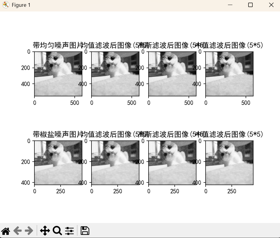
根据运行结果分析可得:
对于均匀噪声,均值滤波、高斯滤波和中值滤波都能在一定程度上降低噪声影响,但都会带来不同程度的模糊,高斯滤波在保留细节方面相对更有优势。
对于椒盐噪声,中值滤波明显优于均值滤波和高斯滤波,是处理椒盐噪声的首选方法,而均值滤波和高斯滤波在处理椒盐噪声时会导致图像严重模糊和失真 。
6.3.2 拓展2
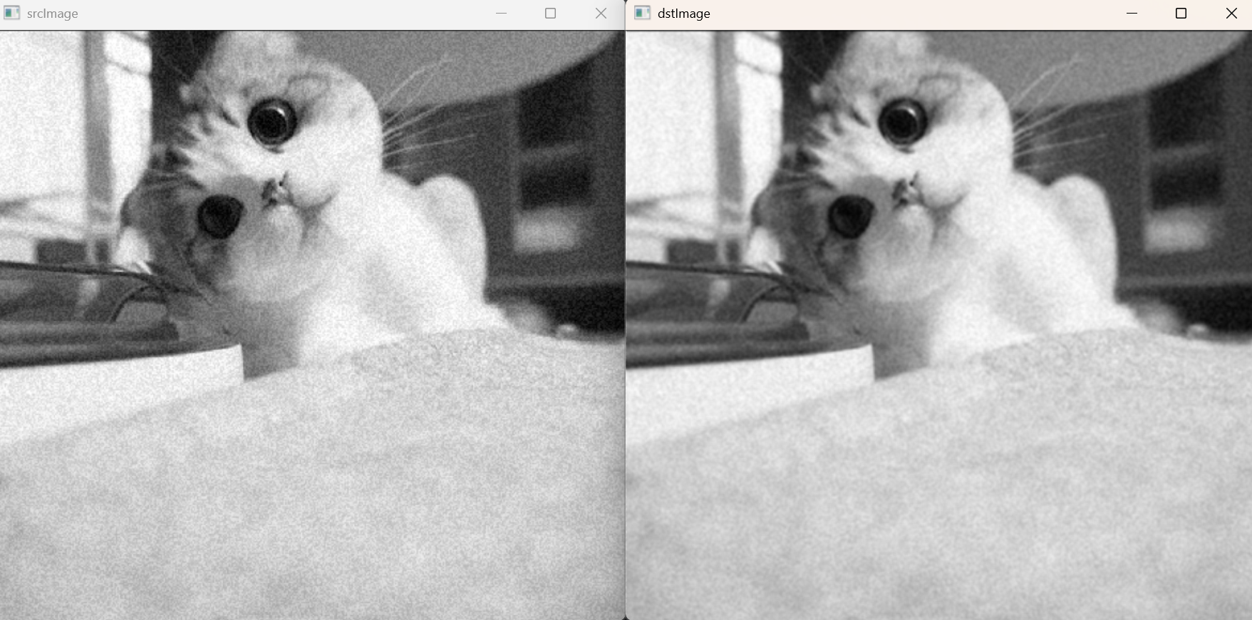
题目:不使用matpolot库,仅使用OpenCV库,来编写均值滤波器和中值滤波器的底层实现代码。对比分析matplot方法与opencv方法的优缺点。
对于拓展2的题目,老师已经给出了均值滤波器的底层实现代码,代码如下及运行结果如图tz2.1。
import cv2


# 求平均
def getAverage(list):
    temp = 0
    for i in list:
        temp = temp + i
    avg = temp / len(list)
    return avg


def main():
    image = cv2.imread('002_u.bmp', 0)
    cv2.imshow('srcImage', image)
# 将tuple中的元素取出,赋值给height,width,channel
    dst = image.copy()
    height = image.shape[0]
    width = image.shape[1]
    # 边界不做处理
    for row in range(1, height - 1):
        for col in range(1, width - 1):
            # 创建一个3✖️3的9阶滤波器
            np = [image[row - 1][col - 1], image[row - 1][col], image[row - 1][col + 1],
                  image[row][col - 1], image[row][col], image[row][col + 1],
                  image[row + 1][col - 1], image[row + 1][col], image[row + 1][col + 1]]
            # 求平均值
            avg = getAverage(np)
            # 给目标图像中对应像素赋灰度值
            dst[row][col] = avg
    cv2.imshow('dstImage', dst)
    cv2.waitKey(0)


if __name__ == '__main__':
    main()
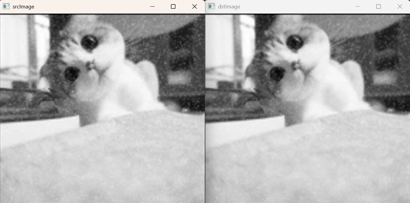
根据老师给出的代码提示,要想编写中值滤波器的底层实现代码,我们只需要将上述代码中的求平均函数修改为求中值函数即可。代码如下及运行结果如图tz2.2。
import cv2


#  求中值
def find_median(numbers):
    # 对列表进行排序
    sorted_numbers = sorted(numbers)
    median = sorted_numbers[len(sorted_numbers) // 2]
    return median


def main():
    image = cv2.imread('002_s.bmp', 0)
    cv2.imshow('srcImage', image)
    dst = image.copy()
    height = image.shape[0]
    width = image.shape[1]
    for row in range(1, height - 1):
        for col in range(1, width - 1):
            np = [image[row - 1][col - 1], image[row - 1][col], image[row - 1][col + 1],
                  image[row][col - 1], image[row][col], image[row][col + 1],
                  image[row + 1][col - 1], image[row + 1][col], image[row + 1][col + 1]]
            # 求中值
            median = find_median(np)
            dst[row][col] = median
    cv2.imshow('dstImage', dst)
    cv2.waitKey(0)


if __name__ == '__main__':
    main()
优点对比:
matpolot:
丰富的绘图功能:Matplotlib是一个强大的绘图库,除了显示图像,还能创建各种类型的图表。可以在一个窗口中同时展示多个图像或图表,并对其进行灵活的布局和标注,方便进行数据分析和可视化。
高质量的图像输出:Matplotlib生成的图像质量较高,支持多种图像格式的保存,并且可以对图像的分辨率、字体、颜色等进行精细的调整。
OpenCV:
高效的图像处理能力:OpenCV专门针对计算机视觉和图像处理任务进行了优化,具有高效的算法实现和底层优化,能够快速处理大规模的图像数据。
丰富的图像处理工具:OpenCV提供了丰富的图像处理工具和算法,包括滤波、边缘检测、特征提取、图像变换等,能够满足各种图像处理需求。
缺点对比:
matpolot:
图像处理功能有限:Matplotlib主要侧重于数据可视化,虽然也能显示图像,但在图像处理方面的功能相对有限。
实时性较差:Matplotlib的绘图操作相对较慢,尤其是在处理大量数据或需要实时更新图像的场景下,可能会出现明显的延迟。
OpenCV:
可视化功能相对较弱:OpenCV的图像显示功能相对简单,主要用于快速查看处理结果,缺乏 Matplotlib那样丰富的绘图和标注功能。


 1571
1571

 被折叠的 条评论
为什么被折叠?
被折叠的 条评论
为什么被折叠?
 到【灌水乐园】发言


