SA与GA求解TSP问题对比分析

Watson_0110

已于 2024-11-12 17:33:58 修改

阅读量659

点赞数 9

文章标签：算法学习方法

于 2024-11-05 19:17:26 首次发布

本文链接：https://blog.youkuaiyun.com/2201_75624332/article/details/143521971

版权

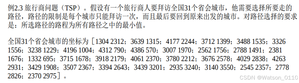
问题：

SA算法：

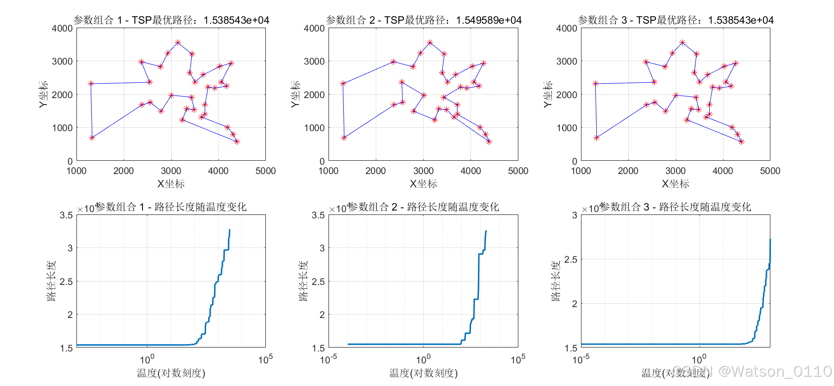
% 定义可调参数的组合
初始温度，终止温度，迭代次数，温度衰减率
param_combinations = [
    3000, 1e-3, 1000, 0.98;  % 参数组合1
    2000, 1e-4, 500, 0.95;   % 参数组合2
    1000, 1e-5, 2000, 0.99   % 参数组合3
];

SA算法
参数组合1 - 最优路径长度：15385.43，运行时间：0.75秒
参数组合2 - 最优路径长度：15495.89，运行时间：0.19秒
参数组合3 - 最优路径长度：15385.43，运行时间：3.58秒

SA算法三种组合参数下的运行结果：

GA算法：

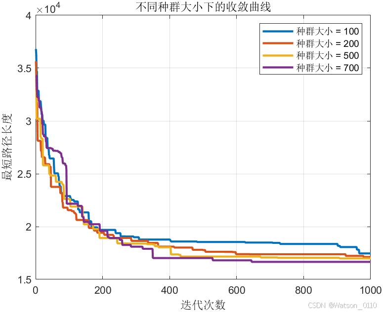
种群大小 = 100 时的运行时间: 0.4080 秒
种群大小 = 200 时的运行时间: 0.8079 秒
种群大小 = 500 时的运行时间: 2.8292 秒
种群大小 = 700 时的运行时间: 4.8889 秒

不同种群大小下的最终最短路径：

    种群大小    最短路径长度
    _______    __________

      100        17463   
      200        17119   
      500        16988   
      700        16662

GA早收敛问题：

GA初始种群降维可视化展示

红色的是SA运行一次初始解降维后的位置，蓝色是GA的初始种群分布！

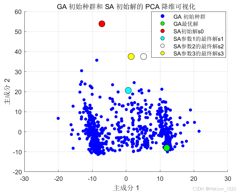
不过值得注意的是，上图反映的仅仅只是生成种群个体的的差异，分布在相邻位置甚至相同位置的个体，并不一定是相同的个体，但是能反映这些个体应该有很强的相关性。同样，哪怕是完全相同的路径，也可能因为出发的城市不同而分布在不同的位置。我们发现这样的个体在二维上分布也有一定距离。

所以，影响GA算法也许和生成的初始种群有很大关系，种群分布太密集可能会降低搜索的效率，造成很多重复个体。浪费搜索空间。

为了进一步探究初始种群对算法的影响，我希望对GA算法引入一个种群个体间的一个距离度量。由于每一个可行解个体，即使是不同的排列方式，也可以得到相同的路径解，因为TSP的解是一个无向环。那么如何去衡量不同解的差异性呢？这里考虑引入一个环形距离的度量：circular_path_distance

function distance = circular_path_distance(path1, path2)
    % 输入为两个种群个体的路径 path1 和 path2，路径长度为31
    % 计算环形路径的距离度量
    
    n = length(path1);  % 假设路径长度为31
    % 初始化距离为一个大的值
    min_distance = inf;
    
    % 遍历所有可能的偏移量（相当于将 path2 旋转来找到最佳匹配）
    for shift = 0:n-1
        % 将 path2 循环移位 shift 个位置
        rotated_path2 = circshift(path2, shift);
        
        % 计算当前移位情况下，path1 和 rotated_path2 的相邻距离之和
        distance_sum = 0;
        for i = 1:n
            % 计算每对相邻城市之间的差异
            distance_sum = distance_sum + abs(path1(i) - rotated_path2(i));
        end
        
        % 更新最小距离
        min_distance = min(min_distance, distance_sum);
    end
    
    % 返回最小的环形路径距离
    distance = min_distance;
end

该算法可以对于GA生成初始种群使进行挑选，确保生成的初始种群能够尽可能分散，通过设置min_distance这个变量作为阈值，判断随机生成的个体是否能够作为初始种群个体之一。这里设置50，得到的如下结果。

但是很遗憾的是，重复多次运行的结果并没有非常明显的提高，还是没有办法找到最优解。也许GA本身的并行特性也决定了它在处理这个TSP问题上，不如SA单个串行求解表现出色。但在求解其他更大规模的计算，遗传算法仍然是非常好的选择，设计初始种群生成策略和适应度函数的计算就非常关键了。在这个问题上我并没有找到一种非常好的设计方式。

SA与GA的算法分析比较

算法的原理差异：首先，明确说明模拟退火（SA）和遗传算法（GA）的搜索策略和优化原理的不同。模拟退火利用逐渐降温的概率接受准则，以确保算法能够跳出局部最优解，朝全局最优解搜索。遗传算法则依赖于种群多样性和遗传操作，但它的进化取决于初始种群的质量。理论上，这种依赖可能导致在初始种群质量不佳时，GA更容易停留在局部最优。
SA的收敛性和全局最优性质：模拟退火的降温过程逐步减少“能量”或“温度”，这与物理中的退火过程类似。根据概率论理论，只要降温足够缓慢，SA能找到全局最优解。引用理论如“大数定理”或马尔可夫链来说明这种收敛性。 GA的多样性瓶颈：遗传算法的理论研究表明，初始种群的多样性对最终解的质量有重要影响。可以引用有关“遗传漂变”（genetic drift）和“收敛加速”的理论来说明，种群过早收敛时，可能导致搜索空间的覆盖不足，进而失去对一些优良解的搜索能力。
实验结果的解释：结合实验数据，可以指出，GA中不同种群规模下的收敛效果与初始种群选择密切相关，而SA由于随机搜索方向的灵活性，其结果波动更小，更具稳定性。理论上，这种一致性支持了SA在TSP问题中更好的求解性能。

结论：

“基于模拟退火逐步降温的接受准则理论支持，SA在TSP中有效跳出局部最优解。”
“GA的进化依赖于多样性保留和适应度选择，理论上更可能因初始种群质量导致收敛到次优解。”

代码：

% 模拟退火算法求解TSP问题，支持多组参数对比
clear;
clc;

% 初始化城市坐标
cities = [
    1304 2312; 3639 1315; 4177 2244; 3712 1399; 3488 1535; 3326 1556;
    3238 1229; 4196 1004; 4312 790; 4386 570; 3007 1970; 2562 1756;
    2788 1491; 2381 1676; 1332 695; 3715 1678; 3918 2179; 4061 2370;
    3780 2212; 3676 2578; 4029 2838; 4263 2931; 3429 1908; 3507 2367;
    3394 2643; 3439 3201; 2935 3240; 3140 3550; 2545 2357; 2778 2826;
    2370 2975
];

% 计算城市间距离矩阵
n = size(cities, 1);
D = zeros(n);
for i = 1:n
    for j = 1:n
        D(i,j) = sqrt((cities(i,1)-cities(j,1))^2 + (cities(i,2)-cities(j,2))^2);
    end
end

% 定义可调参数的组合
param_combinations = [
    3000, 1e-3, 1000, 0.98;  % 参数组合1
    2000, 1e-4, 500, 0.95;   % 参数组合2
    1000, 1e-5, 2000, 0.99   % 参数组合3
];

num_combinations = size(param_combinations, 1);  % 参数组合数量
results = zeros(num_combinations, 1);            % 存储每组参数的最优路径长度
run_times = zeros(num_combinations, 1);          % 存储每组参数的运行时间
paths = cell(num_combinations, 1);               % 存储每组参数的路径
temp_histories = cell(num_combinations, 1);      % 记录温度变化
length_histories = cell(num_combinations, 1);    % 记录路径长度变化

 s = randperm(n);   % 随机排列1到n

for k = 1:num_combinations  % 遍历每组参数组合
    params = struct('T0', param_combinations(k, 1), ...
                    'Tend', param_combinations(k, 2), ...
                    'L', param_combinations(k, 3), ...
                    'q', param_combinations(k, 4));  % 参数结构体

    % 初始化参数
    T = params.T0;  % 当前温度
    count = 0;      % 迭代计数器

    % 产生一个初始解
    % s = randperm(n);   % 随机排列1到n
    s1 = s;            % 当前解
    s2 = s1;           % 新解

    % 记录最优解
    bestS = s1;
    bestL = pathLength(D, s1);
    curL = bestL;

    % 用于记录温度和路径长度的变化
    temp_history = [];     % 记录温度
    length_history = [];   % 记录对应的路径长度

    % 开始计时
    tic;
    
    % 开始模拟退火迭代
    while T > params.Tend
        for j = 1:params.L
            count = count + 1;

            % 产生新解
            p1 = ceil(n * rand);
            p2 = ceil(n * rand);
            if p1 > p2
                tmp = p1;
                p1 = p2;
                p2 = tmp;
            end
            s2 = s1;
            s2(p1:p2) = s1(p2:-1:p1);

            % 计算新解的路径长度
            newL = pathLength(D, s2);

            % Metropolis准则判断是否接受新解
            df = newL - curL;
            if df < 0           % 更好的解，接受
                s1 = s2;
                curL = newL;
                if newL < bestL  % 更新最优解
                    bestS = s2;
                    bestL = newL;
                end
            elseif rand < exp(-df/T)  % 按概率接受差解
                s1 = s2;
                curL = newL;
            end
        end

        % 记录当前温度和对应的最优路径长度
        temp_history = [temp_history T];
        length_history = [length_history bestL];

        % 降温
        T = params.q * T;
    end
    
    % 记录运行时间
    run_times(k) = toc;  % 结束计时并记录时间
    
    % 存储结果
    results(k) = bestL;              % 记录最优路径长度
    paths{k} = bestS;                % 记录最优路径
    temp_histories{k} = temp_history;  % 记录温度变化
    length_histories{k} = length_history;  % 记录路径长度变化

    % 输出每组参数的结果
    fprintf('参数组合%d - 最优路径长度：%.2f，运行时间：%.2f秒\n', k, bestL, run_times(k));
end

% 可视化结果
figure('Position', [100, 100, 1600, 500]);  % 设置图形窗口大小

% 子图1：路径可视化
for k = 1:num_combinations
    subplot(2, num_combinations, k);
    plot(cities(:,1), cities(:,2), 'r*');
    hold on;
    bestS = paths{k};
    for i = 1:n-1
        plot([cities(bestS(i),1), cities(bestS(i+1),1)], ...
             [cities(bestS(i),2), cities(bestS(i+1),2)], 'b-');
    end
    % 连接最后一个城市和第一个城市
    plot([cities(bestS(n),1), cities(bestS(1),1)], ...
         [cities(bestS(n),2), cities(bestS(1),2)], 'b-');
    title(sprintf('参数组合 %d - TSP最优路径：%d', k,results(k)));
    xlabel('X坐标');
    ylabel('Y坐标');
    grid on;
end

% 子图2：路径长度随温度的变化
for k = 1:num_combinations
    subplot(2, num_combinations, num_combinations + k);
    semilogx(temp_histories{k}, length_histories{k}, 'LineWidth', 1.5);
    title(sprintf('参数组合 %d - 路径长度随温度变化', k));
    xlabel('温度(对数刻度)');
    ylabel('路径长度');
    grid on;
end

% 函数定义部分

% 初始化城市坐标
C = [1304 2312; 3639 1315; 4177 2244; 3712 1399; 3488 1535; 3326 1556; ...
    3238 1229; 4196 1044; 4312 790; 4386 570; 3007 1970; 2562 1756 ; ...
    2788 1491; 2381 1676; 1332 695; 3715 1678; 3918 2179; 4061 2370 ; ...
    3780 2212; 3676 2578; 4029 2838; 4263 2931; 3429 1908; 3507 2376 ; ...
    3394 2643; 3439 3201; 2935 3240; 3140 3550; 2545 2357; 2778 2826 ; ...
    2370 2975];
N = size(C, 1);
D = zeros(N);

% 求任意两个城市距离间隔矩阵
for i = 1:N
    for j = 1:N
        D(i, j) = ((C(i, 1) - C(j, 1))^2 + (C(i, 2) - C(j, 2))^2)^0.5;
    end
end

% popSizes = [100, 200, 500, 700]; % 不同的种群规模
G = 1000; % 最大遗传代数

% 初始化保存结果的变量
minDistances = zeros(length(popSizes), G);
finalMinDistances = zeros(length(popSizes), 1);

% % 遍历不同的种群规模
% NP = popSizes(pIdx);
% f = zeros(NP, N);
F = [];

% 参数设置
NP = 700;                % 种群大小
% 生成初始种群
f=generate_initial_population(NP,N,60);

R = f(1:N);
len = zeros(NP, 1);
fitness = zeros(NP, 1);
gen = 0;
Rlength = zeros(G, 1);

% 开始计时
tic;

% 遗传算法循环
while gen < G
    for i = 1:NP
        len(i, 1) = D(f(i, N), f(i, 1));
        for j = 1:N-1
            len(i, 1) = len(i, 1) + D(f(i, j), f(i, j+1));
        end
    end

    maxlen = max(len);
    minlen = min(len);
    rr = find(len == minlen);
    R = f(rr(1, :), :);

    for i = 1:NP
        fitness(i, 1) = 1 - ((len(i, 1) - minlen) / (maxlen - minlen + 0.001));
    end

    nn = 0;
    for i = 1:NP
        if fitness(i, 1) >= rand
            nn = nn + 1;
            F(nn, :) = f(i, :);
        end
    end

    [aa, bb] = size(F);
    while aa < NP
        nnper = randperm(nn);
        A = F(nnper(1), :);
        B = F(nnper(2), :);

        W = ceil(N / 10);
        p = unidrnd(N - W + 1);
        for i = 1:W
            x = find(A == B(p + i - 1));
            y = find(B == A(p + i - 1));
            temp = A(p + i - 1);
            A(p + i - 1) = B(p + i - 1);
            B(p + i - 1) = temp;
            temp = A(x);
            A(x) = B(y);
            B(y) = temp;
        end

        p1 = floor(1 + N * rand());
        p2 = floor(1 + N * rand());
        while p1 == p2
            p1 = floor(1 + N * rand());
            p2 = floor(1 + N * rand());
        end
        tmp = A(p1);
        A(p1) = A(p2);
        A(p2) = tmp;
        tmp = B(p1);
        B(p1) = B(p2);
        B(p2) = tmp;

        F = [F; A; B];
        [aa, bb] = size(F);
    end

    if aa > NP
        F = F(1:NP, :);
    end

    f = F;
    f(1, :) = R;
    clear F;
    gen = gen + 1;
    Rlength(gen) = minlen;
end

% 结束计时并记录时间
elapsedTime = toc;
fprintf('种群大小 = %d 时的运行时间: %.4f 秒\n', NP, elapsedTime);

% 输出每种群规模下的最终最短路径
disp(['不同种群大小下的最终最短路径：',num2str(min(Rlength))]);

% 最优路线图
figure;
for i = 1:N-1
    plot([C(R(i), 1), C(R(i+1), 1)], [C(R(i), 2), C(R(i+1), 2)], 'bo-');
    hold on;
end
plot([C(R(N), 1), C(R(1), 1)], [C(R(N), 2), C(R(1), 2)], 'ro-');
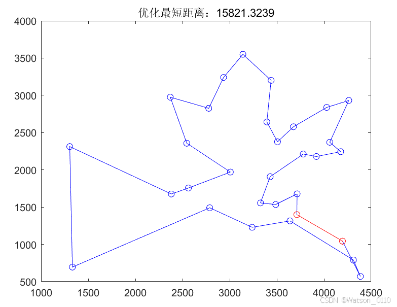
title(['优化最短距离：', num2str(min(Rlength))]);
hold off;

降维种群分布可视化

%PCA降维种群分布可视化
% 假设 F 是 700×31 的初始种群，s1 是 1×31 的 SA 算法初始解

% 将 s1 添加到 F 的最后一行
F_augmented = [f;R;s;paths{1};paths{2};paths{3}];

% 使用 PCA 将 F_augmented 降维到 2 维
[coeff, score, ~] = pca(F_augmented); % 使用 PCA 降维
reducedF_PCA = score(:, 1:2); % 取前两主成分进行可视化

% 可视化 PCA 降维结果
figure;
scatter(reducedF_PCA(1:end-1, 1), reducedF_PCA(1:end-1, 2), 25, 'filled', 'MarkerFaceColor', 'b');
hold on;

% 标出 GA 在降维空间中的位置
scatter(reducedF_PCA(end-4, 1), reducedF_PCA(end-4, 2), 100, 'g', 'filled', 'MarkerEdgeColor', 'k');
% 标出 s 在降维空间中的位置
scatter(reducedF_PCA(end-3, 1), reducedF_PCA(end-3, 2), 100, 'r', 'filled', 'MarkerEdgeColor', 'k');
% 标出 SA最终解在降维空间中的位置
scatter(reducedF_PCA(end-2, 1), reducedF_PCA(end-2, 2), 100, 'c', 'filled', 'MarkerEdgeColor', 'k');
scatter(reducedF_PCA(end-1, 1), reducedF_PCA(end-1, 2), 100, 'w', 'filled', 'MarkerEdgeColor', 'k');
scatter(reducedF_PCA(end, 1), reducedF_PCA(end, 2), 100, 'y', 'filled', 'MarkerEdgeColor', 'k');

title('GA 初始种群和 SA 初始解的 PCA 降维可视化');
xlabel('主成分 1');
ylabel('主成分 2');
legend('GA 初始种群', 'SA 初始解 s','SA参数1的最终解s1','SA参数1的最终解s2','SA参数1的最终解s2','SA参数1的最终解s2' ,'Location', 'best');
grid on;
hold off;

计算城市距离函数||环路距离||生成初始种群函数

function len = pathLength(D, s)
    n = length(s);
    len = D(s(n), s(1));    % 回到起点的距离
    for i = 1:n-1
        len = len + D(s(i), s(i+1));
    end
end
function distance = circular_path_distance(path1, path2)
    % 输入为两个种群个体的路径 path1 和 path2，路径长度为31
    % 计算环形路径的距离度量
    
    n = length(path1);  % 假设路径长度为31
    % 初始化距离为一个大的值
    min_distance = inf;
    
    % 遍历所有可能的偏移量（相当于将 path2 旋转来找到最佳匹配）
    for shift = 0:n-1
        % 将 path2 循环移位 shift 个位置
        rotated_path2 = circshift(path2, shift);
        
        % 计算当前移位情况下，path1 和 rotated_path2 的相邻距离之和
        distance_sum = 0;
        for i = 1:n
            % 计算每对相邻城市之间的差异
            distance_sum = distance_sum + abs(path1(i) - rotated_path2(i));
        end
        
        % 更新最小距离
        min_distance = min(min_distance, distance_sum);
    end
    
    % 返回最小的环形路径距离
    distance = min_distance;
end

function population = generate_initial_population(popSize, numCities, minDistance)
    % popSize 是种群规模
    % numCities 是城市数量（如31）
    % minDistance 是每个新个体与已有个体之间的最小距离要求
    population = zeros(popSize, numCities);  % 初始化种群
    population(1, :) = randperm(numCities);  % 随机生成第一个个体

    for i = 2:popSize
        while true
            % 随机生成一个新的路径（个体）
            candidate = randperm(numCities);
            
            % 计算该候选个体与已有种群中所有个体的距离
            valid = true;
            for j = 1:i-1
                dist = circular_path_distance(candidate, population(j, :));
                if dist < minDistance
                    valid = false;
                    break;  % 如果距离不满足要求，则重新生成该候选个体
                end
            end
            
            % 如果满足距离要求，则将该个体添加到种群中
            if valid
                population(i, :) = candidate;
                break;
            end
        end
    end
end