使用OpenCV进行SVM分类demo

代码来源 https://github.com/mbeyeler/opencv-machine-learning/blob/master/notebooks/06.01-Implementing-Your-First-Support-Vector-Machine.ipynb

from sklearn import datasets
import cv2
import matplotlib.pyplot as plt
import numpy as np
from sklearn import model_selection as ms
from sklearn import metrics

X, y = datasets.make_classification(n_samples=100, n_features=2,
                                    n_redundant=0, n_classes=2,
                                    random_state=7816)

plt.style.use('ggplot')
plt.set_cmap('jet')

plt.figure(figsize=(10, 6))
plt.scatter(X[:, 0], X[:, 1], c=y, s=100)
plt.xlabel('x values')
plt.ylabel('y values')

X = X.astype(np.float32)
y = y * 2 - 1

X_train, X_test, y_train, y_test = ms.train_test_split(
    X, y, test_size=0.2, random_state=42
)

def plot_decision_boundary(svm, X_test, y_test):
    # create a mesh to plot in
    h = 0.02  # step size in mesh
    x_min, x_max = X_test[:, 0].min() - 1, X_test[:, 0].max() + 1
    y_min, y_max = X_test[:, 1].min() - 1, X_test[:, 1].max() + 1
    xx, yy = np.meshgrid(np.arange(x_min, x_max, h),
                         np.arange(y_min, y_max, h))
    
    X_hypo = np.c_[xx.ravel().astype(np.float32),
                   yy.ravel().astype(np.float32)]
    _, zz = svm.predict(X_hypo)
    zz = zz.reshape(xx.shape)
    
    plt.contourf(xx, yy, zz, cmap=plt.cm.coolwarm, alpha=0.8)
    plt.scatter(X_test[:, 0], X_test[:, 1], c=y_test, s=200)

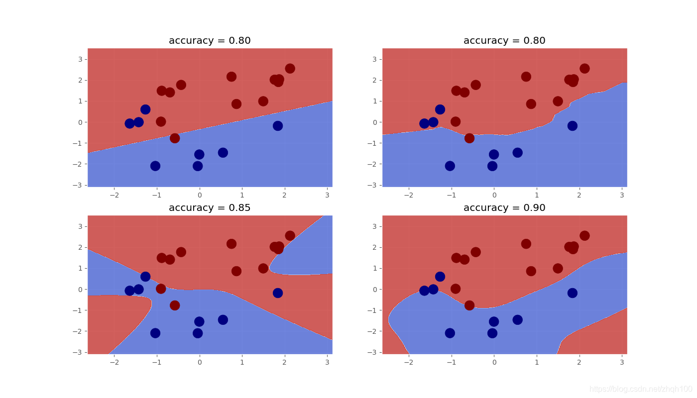
kernels = [cv2.ml.SVM_LINEAR, cv2.ml.SVM_INTER, cv2.ml.SVM_SIGMOID, cv2.ml.SVM_RBF]

plt.figure(figsize=(14, 8))
for idx, kernel in enumerate(kernels):
    svm = cv2.ml.SVM_create()
    svm.setKernel(kernel)
    svm.train(X_train, cv2.ml.ROW_SAMPLE, y_train)
    _, y_pred = svm.predict(X_test)
    
    plt.subplot(2, 2, idx + 1)
    plot_decision_boundary(svm, X_test, y_test)
    plt.title('accuracy = %.2f' % metrics.accuracy_score(y_test, y_pred))
plt.show()

结果如下：