人工神经网络实现三阶贝塞尔曲线拟合散点

一、背景

        之前做过一个项目是需要将位图转换成矢量图，其中一个很重要的步骤，就是需要用贝塞尔曲线拟合一些散列点。了解贝塞尔曲线的同学都知道，如果贝塞尔曲线的控制点都明确的情况下，想算出来线上的点是很容易的，直接套公式就可以把点的坐标算出来。但是如果这个过程反过来，给你一些点的坐标，求出贝塞尔曲线的控制点，是很困难的。

        三阶贝塞尔曲线的公式： P = P0*(1-t)**3 + 3*P1*t*(1-t)**2 + 3*P2*t**2*(1-t) + P3*t**3 (公式中*表示乘法运算，**表示幂运算)

二、思路

       1、用圆拟合散点，再用三阶贝塞尔曲线拟合圆。优点算法简单，缺点，曲线很僵硬，放大看全是圆弧，失去了贝塞尔曲线的强大的表达能力。

       2、用二阶贝塞尔曲线拟合散点，优点算法简单，运算效率高。缺点二阶贝塞尔曲线实际就是抛物线，表达能力有限和思路1类似。

       3、用最小二乘法。优点运算可靠，速度快。缺点，公式推导复杂，理解很难。方法很可取，但是不是本文讲述的重点。

       4、网上搜了很多，有用遗传算法的，各种。后来想想，目前这么火热的人工神经网络能否解决这个问题呢？本文带大家一起尝试一下。

三、尝试

      试着用人工神经网络来搞定这个问题。就要考虑输入输出。

      1、输入，输入肯定是散列点。但是怎么输入呢，人工神经网络大部分输入参数都是固定的，但是散列点根据线的长度，个数不固定。能否想办法固定下来呢？我们选一些代表性的点，起点、终点、三个四分之一点。总共5个点，10个值。

      2、输出，输出控制点的坐标。起点、终点已知、那么就要两个控制点的坐标，总共4个数字。那么输出就是4个值。

四、网络搭建

       本次网络不牵涉到图像运算，就采用双隐藏层的ANN网络即可解决问题。网络结构很简单，读者可自行搜索。这里不做详细介绍，后面直接上代码。

五、数据集

       数据集自己写随机代码生成即可，放在训练过程中，可以做成无监督学习，省时省力。

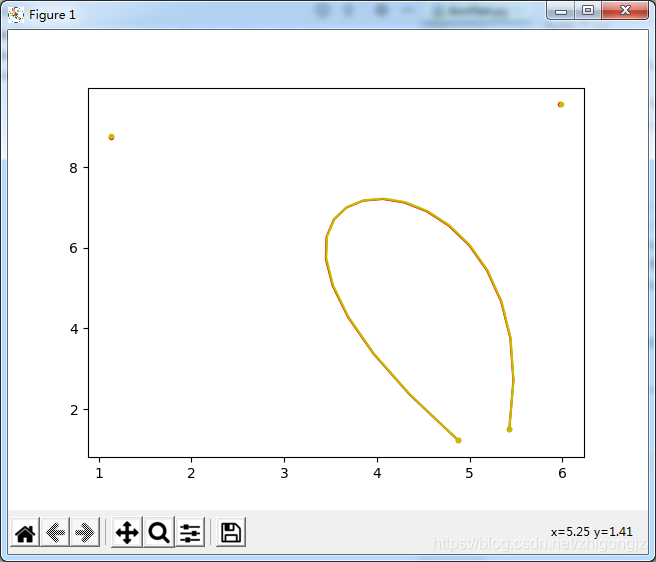
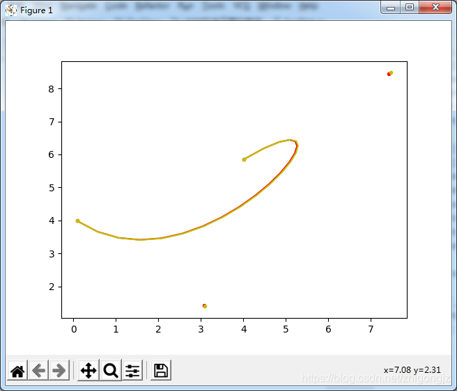
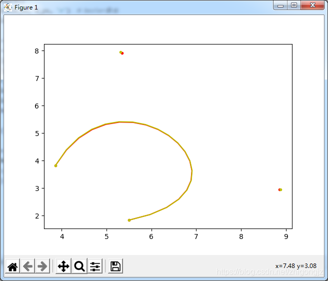
六、实验效果。

       直接上图，图中红色点是实际控制点，黄色点是网络预测的点，几乎重合，曲线也几乎重合，效果很好：

七、代码

tensorflow 2.0+，如果对您有用，请帮忙点赞哈，文章是原创，转载请标明出处，沟通交流加我QQ306128847,。

import tensorflow as tf
from tensorflow.keras import layers, models
from matplotlib import pyplot as plt
import numpy as np
import os

b_xs = []
b_ys = []
# xs表示原始数据
# n表示阶数
# k表示索引
def one_bezier_curve(a, b, t):
    return (1 - t) * a + t * b


def n_bezier_curve(xs, n, k, t):
    if n == 1:
        return one_bezier_curve(xs[k], xs[k + 1], t)
    else:
        return (1 - t) * n_bezier_curve(xs, n - 1, k, t) + t * n_bezier_curve(xs, n - 1, k + 1, t)

def bezier_curve(xs, ys, num, b_xs, b_ys):
    n = 3  # 采用5次bezier曲线拟合
    t_step = 1.0 / (num - 1)
    # t_step = 1.0 / num
    print(t_step)
    t = np.arange(0.0, 1 + t_step, t_step)
    print(len(t))
    for each in t:
        b_xs.append(n_bezier_curve(xs, n, 0, each))
        b_ys.append(n_bezier_curve(ys, n, 0, each))

class AnnNet(object):
    def __init__(self):
        model = models.Sequential()
        model.add(layers.Dense(64, activation='sigmoid', input_shape=(10,)))
        model.add(layers.Dense(32, activation='sigmoid'))
        model.add(layers.Dense(4))
        model.summary()
        self.model = model

    def GenerateArray(self):
        while 1:
            x= []
            y= []
            for i in range(10):
                point = np.random.rand(8) * 10
                times = np.random.rand(3)
                times = [0.2, 0.5, 0.8]
                pt1x = ((1 - times[0]) ** 3) * point[0] + 3 * times[0] * ((1 - times[0]) ** 2) * point[2]  + 3 * (times[0] ** 2) * (1 - times[0]) * point[4] + (times[0] ** 3) * point[6]
                pt1y = ((1 - times[0]) ** 3) * point[1] + 3 * times[0] * ((1 - times[0]) ** 2) * point[3]  + 3 * (times[0] ** 2) * (1 - times[0]) * point[5] + (times[0] ** 3) * point[7]
                pt2x = ((1 - times[1]) ** 3) * point[0] + 3 * times[1] * ((1 - times[1]) ** 2) * point[2]  + 3 * (times[1] ** 2) * (1 - times[1]) * point[4] + (times[1] ** 3) * point[6]
                pt2y = ((1 - times[1]) ** 3) * point[1] + 3 * times[1] * ((1 - times[1]) ** 2) * point[3]  + 3 * (times[1] ** 2) * (1 - times[1]) * point[5] + (times[1] ** 3) * point[7]
                pt3x = ((1 - times[2]) ** 3) * point[0] + 3 * times[2] * ((1 - times[2]) ** 2) * point[2]  + 3 * (times[0] ** 2) * (1 - times[2]) * point[4] + (times[2] ** 3) * point[6]
                pt3y = ((1 - times[2]) ** 3) * point[1] + 3 * times[2] * ((1 - times[2]) ** 2) * point[3]  + 3 * (times[0] ** 2) * (1 - times[2]) * point[5] + (times[2] ** 3) * point[7]
                x.append([point[0], point[1], pt1x, pt1y, pt2x, pt2y, pt3x, pt3y, point[6], point[7]])
                y.append([point[2], point[3], point[4], point[5]])
            X = np.array(x)
            Y = np.array(y)
            yield (X, Y)

    def LossFunc(self, ytrue, ypred):
        loss = tf.reduce_mean(tf.square(ytrue-ypred))
        return loss

    def Train(self):
        print('train start!')
        self.check_path = 'save.ckpt'
        if os.path.exists(self.check_path + '.index'):
            self.model.load_weights(self.check_path)
        self.model.compile(optimizer='adam', loss = self.LossFunc)
        save_model_cb = tf.keras.callbacks.ModelCheckpoint(self.check_path, save_weights_only=True, verbose=1, period=1)
        back = self.model.fit_generator(self.GenerateArray(), steps_per_epoch=1000, epochs=100, callbacks=[save_model_cb])
        print('train end!')

    def Test(self):
        print('test start!')
        self.check_path = 'save.ckpt'
        if os.path.exists(self.check_path + '.index'):
            self.model.load_weights(self.check_path)
        x= []
        y= []
        point = np.random.rand(8) * 10
        times = [0.2, 0.5, 0.8]
        pt1x = ((1 - times[0]) ** 3) * point[0] + 3 * times[0] * ((1 - times[0]) ** 2) * point[2]  + 3 * (times[0] ** 2) * (1 - times[0]) * point[4] + (times[0] ** 3) * point[6]
        pt1y = ((1 - times[0]) ** 3) * point[1] + 3 * times[0] * ((1 - times[0]) ** 2) * point[3]  + 3 * (times[0] ** 2) * (1 - times[0]) * point[5] + (times[0] ** 3) * point[7]
        pt2x = ((1 - times[1]) ** 3) * point[0] + 3 * times[1] * ((1 - times[1]) ** 2) * point[2]  + 3 * (times[1] ** 2) * (1 - times[1]) * point[4] + (times[1] ** 3) * point[6]
        pt2y = ((1 - times[1]) ** 3) * point[1] + 3 * times[1] * ((1 - times[1]) ** 2) * point[3]  + 3 * (times[1] ** 2) * (1 - times[1]) * point[5] + (times[1] ** 3) * point[7]
        pt3x = ((1 - times[2]) ** 3) * point[0] + 3 * times[2] * ((1 - times[2]) ** 2) * point[2]  + 3 * (times[0] ** 2) * (1 - times[2]) * point[4] + (times[2] ** 3) * point[6]
        pt3y = ((1 - times[2]) ** 3) * point[1] + 3 * times[2] * ((1 - times[2]) ** 2) * point[3]  + 3 * (times[0] ** 2) * (1 - times[2]) * point[5] + (times[2] ** 3) * point[7]
        x.append([point[0], point[1], pt1x, pt1y, pt2x, pt2y, pt3x, pt3y, point[6], point[7]])
        y.append([point[2], point[3], point[4], point[5]])
        X = np.array(x)
        Y = np.array(y)
        ypred = self.model.predict(X)
        print(Y)
        print(ypred)
        num = 20
        xs = [point[0], point[2], point[4], point[6]]
        ys = [point[1], point[3], point[5], point[7]]
        b_xs = []
        b_ys = []
        bezier_curve(xs, ys, num, b_xs, b_ys)  # 将计算结果加入到列表中
        plt.figure()
        plt.plot(b_xs, b_ys, 'r')  # bezier曲线
        plt.plot(xs, ys, '.r')  # 控制点

        b_xs = []
        b_ys = []
        xs = [point[0], ypred[0][0], ypred[0][2], point[6]]
        ys = [point[1], ypred[0][1], ypred[0][3], point[7]]
        bezier_curve(xs, ys, num, b_xs, b_ys)  # 将计算结果加入到列表中
        plt.plot(b_xs, b_ys, 'y')  # bezier曲线
        plt.plot(xs, ys, '.y')  # 控制点
        plt.show()

        print('test end!')

if __name__ == '__main__':
    net = AnnNet()
    net.Train()
    net.Test()